Translate this page into:
A numerical method for a delayed viral infection model with general incidence rate
⁎Corresponding author. k.hattaf@yahoo.fr (Khalid Hattaf)
-
Received: ,
Accepted: ,
This article was originally published by Elsevier and was migrated to Scientific Scholar after the change of Publisher.
Peer review under responsibility of King Saud University.
Abstract
In this paper, we construct a numerical method for a delayed viral infection model with general incidence rate. We prove that the obtained discrete model has the same dynamics as the corresponding continuous model, such as positivity, boundedness and global behaviors of solutions with no restriction on the time step size. Furthermore, numerical simulations are given to illustrate and confirm our main analytical results.
Keywords
Delay difference equations
General incidence rate
Mixed Euler method
Global stability
1 Introduction
In recent years, several authors are interested in the study of the dynamics of viral infections by proposing the continuous mathematical models with delays and different forms of incidence rate, such as mass action process (Zhu and Zou, 2008; Li and Shu, 2010; Hattaf and Yousfi, 2011; Vargas-De-León, 2012), standard incidence function (Gourley et al., 2008; Eikenberry et al., 2009; Tian and Xu, 2010), saturated mass action (Li and Ma, 2007; Xu, 2011), Beddington–DeAngelis functional response (Huang et al., 2011; Xiang et al., 2013) and Crowley–Martin functional response (Zhou and Cui, 2011). In 2013, the authors (Hattaf et al. (2013)) have generalized all previous forms by proposing the following model:
From the biological point of view, the three hypotheses are reasonable. Indeed, the first means that the incidence rate is equal to zero if there are no susceptible cells. The second one signifies that the incidence rate is increasing when the numbers of infected cells and virus are constant and the number of susceptible cells increases. Hence, the second hypothesis means the more the amount of susceptible cells, the more the average number of cells which are infected by each virus in the unit time will occur. Similarly, the third assumption means the more the amount of infected cells or virus, the less the average number of cells which are infected by each virus in the unit time will be. On the other hand, the infectious process is not instantaneous. For this reason, we choose to use delay differential equations in order to take into account the time needed for infected cells to produce new virions after viral entry and the time necessary for the newly produced virions to become mature and infectious.
In Hattaf et al. (2013), Hattaf et al. proved the positivity and boundedness of solutions. Also, they identified the basic reproduction number of model (1) as follows Moreover, they established the global stability of equilibria.
In reality, scientists often collect the data and analyze the results at discrete times. In addition, the numerical simulations of continuous models are obtained by discretizing these models. For these reasons, we will discretize the model (1) by using ‘mixed’ Euler method which is a mixture of both forward and backward Euler methods. Furthermore, we will show that the discrete model obtained by the mixed Euler method maintains essential dynamical properties, such as positivity, boundedness and global behaviors of solutions with no restriction on the time step size.
The remainder of this paper is organized as follows. In the next section, we introduce our discrete virus dynamics model with general and two delays, and establish some preliminary results. The stability of the disease-free equilibrium and the chronic infection equilibrium of the new delayed discrete model is investigated in Sections 3 and 4. Numerical simulations are given to verify the main theoretical results in Section 5. The paper ends with a conclusion in Section 6.
2 Delayed discrete model and preliminaries
Let h be a time step size. Assume that there exist integers
with
and
. The grids points are
for
. By applying both forward and backward Euler methods and using the approximations
and
, we obtain the following delayed discrete model
The following result establishes the positivity and boundedness of solutions of the discrete model (2).
All solutions of system (2) subject to condition (3) remain nonnegative and bounded for all .
First, we prove the positivity of solutions by using mathematical induction. When , we have Let . Clearly, g(x) is a continuous function for and Then is monotonically increasing on . Hence, the equation has a unique solution on . Since we have . Hence, . From (2), we obtain Then and . Therefore, by using the induction, we get and for all . This proves the positivity of solutions.
Next, we prove the boundedness of solutions. Let Then, where . Hence, By using the induction, we get the following inequality Then, This implies that is bounded. Therefore, and are also bounded.
By the third equation of (2), we obtain As is bounded, then there exists a M such that for all . Thus, By induction, we get Therefore, is bounded. This completes the proof. □
If in addition we assume that and , it is easy to get the following result.
If and , then all solutions of system (2) subject to condition (3) are positive for any . In this case, the mixed Euler numerical scheme for the system (1) is called unconditionally positive.
Next, we find the steady states of system (2). By a simple computation, it is easy to see that the system (2) has the same steady states as those of the corresponding continuous system (1).
3 Stability of the disease-free equilibrium
In this section, we investigate the stability of the disease-free equilibrium.
The disease-free equilibrium of system (2) is globally asymptotically stable whenever , and unstable otherwise.
We construct a discrete Lyapunov functional as follows Calculating the first difference of along the positive solution of system (2), we have Using the equality , we get Since is strictly monotonically increasing with respect to x, we have Since , we have for all . Then, is a monotonically decreasing sequence. Since , we have . Hence , from which we obtain and . We discuss two cases:
-
If , then . By the third equation of (2), we get .
-
If . Using and the first equation of (2), it is not hard to have .
Now, we prove that the disease-free equilibrium
is unstable when
. Calculating the linearization system of model (2) at equilibrium
, we get a new system of the form
We have and P is a continuous function on interval . Then there exists a such that . Therefore, is unstable when . This completes the proof. □
4 Stability of the chronic infection equilibrium
In this section, we establish the global stability of the chronic infection equilibrium
, by assuming that
and the function f satisfies the following hypothesis
The assumption (H4) is satisfied by various types of the incidence rate including the mass action when , the saturation incidence when , the incidence function was used in Zhuo (2012) and Sun and Min (2014) when , Beddington–DeAngelis response when , Crowley-Martin response when and the more generalized response introduced by Hattaf et al. (see Section 5 in Hattaf et al. (2013)) when , where is a positive constant rate describing the infection process, and are nonnegative constants. Further, the fourth hypothesis given in Wang et al. (2013) on the incidence function depending only of x and v is a particular case of the assumption (H4).
The following theorem establish the global stability of .
Assume and (H4) hold. Then the chronic infection equilibrium of system (2) is globally asymptotically stable.
We define a discrete Lyapunov functional as follows where . Clearly, attains its strict global minimum at and .
The function has the global minimum at and . So, for all . Thus, with equality holding if and only if for all .
The first difference of satisfies By the inequality , we get Using and , we obtain Since is strictly monotonically increasing with respect to x, we obtain that According to (H4), we have Since for , we deduce that for all . Then, is a monotonically decreasing sequence. Since , it follows that . Hence, we obtain that , which implies that and . From system (2), we obtain and . Therefore, we conclude that is globally asymptotically stable. □
5 Numerical simulations
In this section, we will confirm and illustrate our previous theoretical results by numerical simulations. For this, we consider the following delayed discrete model for HIV infection:
Firstly, we simulate the model (6) by using the following parameter values: λ = 10 cells mm−3 day−1 (Perelson et al., 1993), d = 0.02 day−1 (Perelson et al., 1993), a = 0.5 day−1 (Perelson et al., 1996), u = 3 day−1 (Perelson et al., 1996), β = 0.000024 mm3 virion−1 day−1 (Perelson et al., 1996; Stafford et al., 2000),
(Perelson et al., 1993), k = 600 virions cell−1 day−1 (Hattaf and Yousfi, 2012) α2 = 0.65 day−1, τ1 = 3.5 days, τ2 = 2.5 days and h = 0.1 days. By calculating, we have
. By Theorem 3.1, we deduce that the disease-free equilibrium
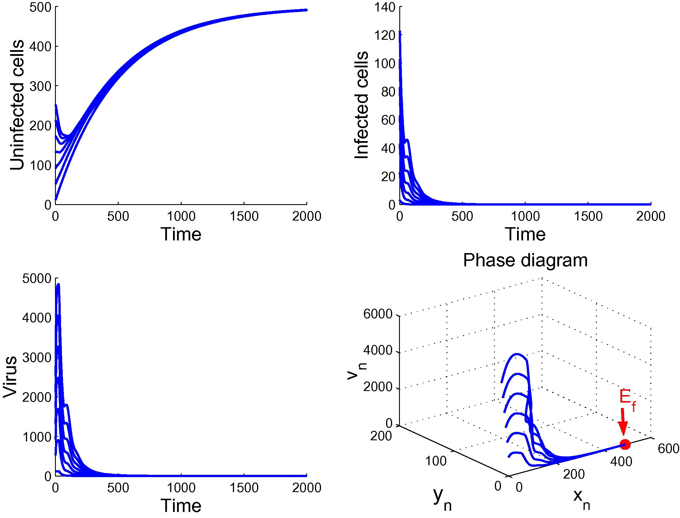
of (6) is globally asymptotically stable, which means that the virus is cleared and the infection dies out. Fig. 1 validates the above analysis.
Plot demonstrates the global stability of
.
Secondly, we choose β = 0.00024 mm3 virion−1 day−1 (Perelson et al., 1996; Stafford et al., 2000) and the other parameter values are the same as above. The reason to just modify the parameter
is based on the fact that
is an increasing function with respect to
(see the explicit formula (7) for
). By calculating, we have
. Then, system (6) has a unique chronic infection equilibrium
. By applying Theorems 3.1 and 4.2, we see that
becomes unstable and
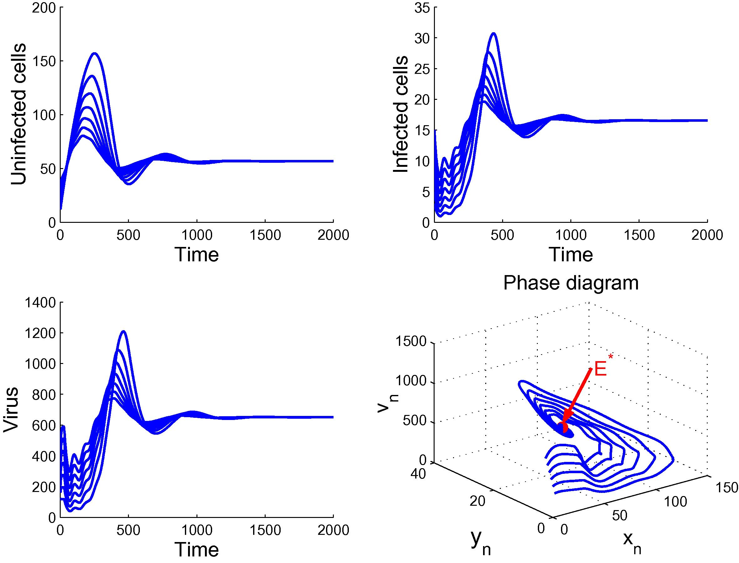
is globally asymptotically stable. In this case, the virus persists in the host and the infection becomes chronic. Fig. 2 confirms this observation.
Plot demonstrates the global stability of
.
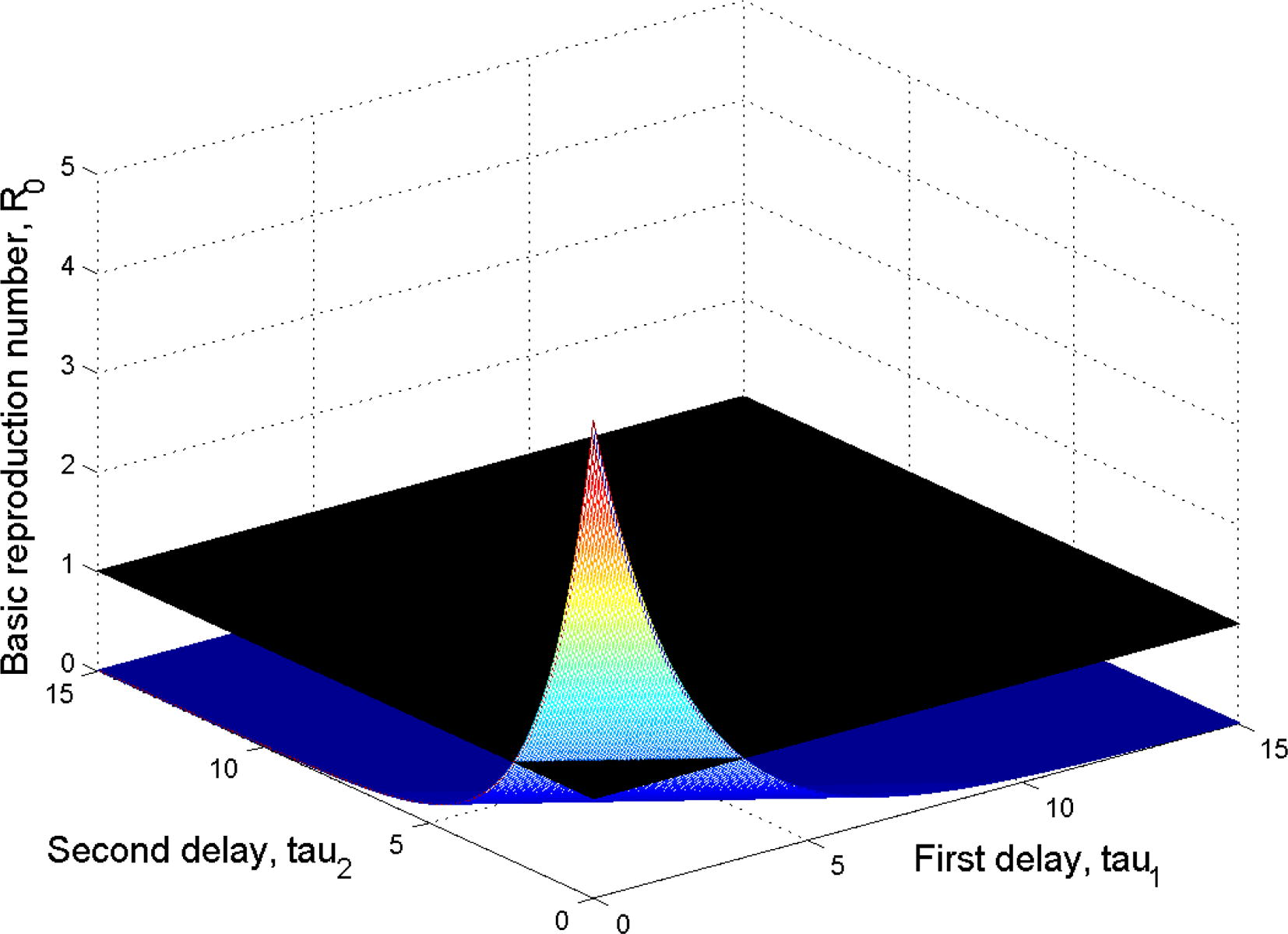
According to the above, we deduce a strategy to control the viral infection. This strategy is based on reducing the value of
and making it less than or equal to one. From the explicit expression of
in (7), it is clear that with the increase in time delays
and
, the value of
decreases which is demonstrated in Fig. 3.
Plot of the basic reproduction number
as a function of the time delays
and
.
6 Conclusion
In this work, we have proposed a discrete mathematical model with two delays to describe the dynamics of viral infection, such as human immunodeficiency virus (HIV), the hepatitis B virus (HBV) and the hepatitis C virus (HCV). The discrete model is derived from the continuous system (1) by using a mixed Euler method. Also, the infection transmission process is modeled by a general incidence function that includes various types of incidence rate existing in the literature. We have proved that the proposed mixed Euler method is unconditionally positive. Furthermore, the dynamical behaviors of the the delayed discrete model are investigated by linearization method and by constructing suitable discrete Lyapunov functionals. More precisely, we have proved that the disease-free equilibrium is globally asymptotically stable if the basic reproduction number satisfies , which means that the virus is cleared and the infection dies out. When becomes unstable and the chronic infection equilibrium is globally asymptotically stable. In this case, the virus persists in the host and the infection becomes chronic. Therefore, we conclude that the discrete model has the same qualitative properties as the corresponding continuous viral infection model (1) with no restriction on the time step size.
Acknowledgement
We would like to thank the editor and anonymous referees for their very helpful comments and suggestions that greatly improve the presentation of this work.
References
- The dynamics of a delay model of HBV infection with logistic hepatocyte growth. Math. Biosci. Eng.. 2009;6:283-299.
- [Google Scholar]
- Dynamics of a delay differential model of hepatitis B virus. J. Biol. Dyn.. 2008;2:140-153.
- [Google Scholar]
- A delay differential equation model of HIV with therapy and cure rate. Int. J. Nonlinear Sci.. 2011;12:503-512.
- [Google Scholar]
- Two optimal treatments of HIV infection model. World J. Model. Simul.. 2012;8(1):27-35.
- [Google Scholar]
- Global stability of a virus dynamics model with cure rate and absorption. J. Egypt. Math. Soc.. 2014;22(2014):386-389.
- [Google Scholar]
- Mathematical analysis of a virus dynamics model with general incidence rate and cure rate. Nonlinear Anal. RWA. 2012;13:1866-1872.
- [Google Scholar]
- Stability analysis of a virus dynamics model with general incidence rate and two delays. Appl. Math. Comput.. 2013;221:514-521.
- [Google Scholar]
- A Delay virus dynamics model with general incidence rate. Differ. Equ. Dyn. Syst.. 2014;22(2):181-190.
- [Google Scholar]
- Global analysis for delay virus dynamics model with Beddington–DeAngelis functional response. Appl. Math. Lett.. 2011;24(7):1199-1203.
- [Google Scholar]
- Asymptotic properties of an HIV-1 infection model with time delay. J. Math. Anal. Appl.. 2007;335:683-691.
- [Google Scholar]
- Global dynamics of an in-host viral model with intracellular delay. Bull. Math. Biol.. 2010;72:1492-1505.
- [Google Scholar]
- HIV-1 dynamics in vivo: virion clearance rate, infected cell life-span, and viral generation time. Science. 1996;271:1582-1586.
- [Google Scholar]
- Modeling plasma virus concentration during primary HIV infection. J. Theor. Biol.. 2000;203(3):285-301.
- [Google Scholar]
- Dynamics analysis and simulation of a modified HIV infection model with a saturated infection rate. Computat. Math. Methods Med.. 2014;2014
- [CrossRef] [Google Scholar]
- Asymptotic properties of a hepatitis B virus infection model with time delay. Disc. Dyn. Nat. Soc. 2010 21 pages
- [CrossRef] [Google Scholar]
- Stability analysis of a model for HBV infection with cure of infected cells and intracellular delay. Appl. Math. Computat.. 2012;219:389-398.
- [Google Scholar]
- Global stability analysis for delayed virus infection model with general incidence rate and humoral immunity. Math. Comput. Simul.. 2013;89:13-22.
- [Google Scholar]
- Stability of the virus dynamics model with Beddington–DeAngelis functional response and delays. Appl. Math. Model.. 2013;37:5414-5423.
- [Google Scholar]
- Global stability of an HIV-1 infection model with saturation infection and intracellular delay. J. Math. Anal. Appl.. 2011;375:75-81.
- [Google Scholar]
- Global stability of the viral dynamics with Crowley–Martin functional response. Bull. Korean Math. Soc.. 2011;48:555-574.
- [Google Scholar]
- Impact of delays in cell infection and virus production on HIV-1 dynamics. Math. Med. Biol.. 2008;25:99-112.
- [Google Scholar]
- Analysis of a HBV infection model with non-cytolytic cure process. IEEE 6th Int. Conf. Syst. Biol. 2012:148-151.
- [Google Scholar]


