Adaptive control of inventory systems with unknown deterioration rate

1 Introduction

Applications of optimal control theory to management science, in general, and to production planning, in particular, are proving to be quite fruitful; see Sethi and Thompson (2000). Naturally, with the optimal control theory, optimal control techniques came to be applied to production planning problems. For example,

• Self-tuning control: Hedjar et al. (2007) study how to use control and identification methods for controlling the system when its parameters are not all a priori known to the designer.

• Receding-horizon control: Hedjar et al. (2005) applied a discrete-time technique in which the control action is obtained by repeatedly solving on-line open-loop optimization problems at each time step.

• Predictive control: Hedjar et al. (2004) used a j-step ahead predictor to predict the tracking error. An identification algorithm is incorporated to estimate the model parameters in the case where they are unknown.

In this paper we apply yet another optimal control technique, called model reference adaptive control (MRAC), in which the performance specifications are given in terms of a model (or targets, or goals); see for example Sastry and Bodson (1989). The goals represent the ideal state of the process. Adaptive control is therefore similar to self-tuning control in that it also attempts to overcome unknown or varying system dynamics while achieving adequate tracking performances.

In order to apply the MRAC to the problem of production planning, we will be using another concept from optimal control theory that of feedback control. This concept was first applied by James Watt to control the speed of his steam engine about 200 years ago. Since then, the number of industrial applications has increased to the point that most automatic control systems today include feedback control. As we progress, we will occasionally make use of some notions from the theory of optimal control that may not be familiar to the management scientists. Each time this proves to be necessary, we will be giving, for the novice, the definition of such notions. In the next section we introduce the notation and formally describe the system. We are assuming that the firm of interest to us adopts a continuous-review (instead of a periodic-review) policy. In Section 3 we derive the optimal control variable when all system parameters are known while in Section 4, we derive the optimal control variable when not all system parameters are known. Illustrative examples are provided in both Sections 3 and 4.

2 Model assumptions and notation

We consider the classical production planning problem in which a manufacturing firm producing a single item, selling some and stocking the remaining units. We assume that the firm has set an inventory goal level and a production (or control) goal rate. We also assume that a proportion of the units in stock deteriorate at a constant rate which may be known or unknown. Item deterioration is of great importance in inventory theory see Goyal and Giri (2001). In this paper, we apply an optimal control technique, called model reference adaptive control (MRAC) to the fore cited production planning problem where the firm adopts a continuous-review policy, that is, the inventory level is monitored continuously. To state the model we use the following notation:

• I(t): inventory level at time t,

• P(t): production rate at time t (P(t) ⩾ 0),

• D(t): demand rate at time t,

• θ: constant deterioration rate (θ > 0),

• I_d(t): inventory goal level at time t,

• P_d(t): production goal rate at time t (P_d(t) ⩾ 0).

The interpretation of the goal rates is as follows:

• The inventory goal level I_d(t) is a safety stock that the firm wants to keep on hand at time t.

• The production goal rate P_d(t) is the most efficient rate desired by the firm at time t.

Given a reference model in terms of goals I_d for the inventory level I (state variable) and P_d for the production rate P, the objective of the control problem is to choose an appropriate production rate P such that all the functions involved are bounded and I tracks I_d.

Since demand occurs at rate D, production occurs at the controllable rate P, and deterioration occurs at a constant rate θ, it follows that the inventory level I evolves at each instant of time t according to the state equation

In the analysis of process dynamics, the process variables and controls are functions of the time t.

Taking the Laplace transform of both sides of (2.3), we have:

The parameter a_d, which is chosen to be positive (a_d > 0) in order to ensure the stability of the reference model, represents the rate of convergence of the desired inventory level.

Since the final value of the desired inventory level is given by: ${\lim }_{t\to \infty }{I}_d(t)=\frac{b_d}{a_d}{u}_d(t)$ or $I_d(\infty )=\frac{b_d}{a_d}{u}_d(\infty )$ . One can choose the parameter b_d to tune the gain $\frac{b_d}{a_d}$ between the input/output of the reference model. The parameter b_d is also chosen to be positive (b_d > 0) in order to preserve the sign between the input and the output of the reference model.

Further, the form of Eq. (2.4) allows us to break the transform of the output variable (namely the desired inventory level I_d) into the product of two terms: the fraction, known as the transfer function, and the transform of the input variable (namely the desired production rate u_d). The transfer function and its parameters characterize the process and determine how the output variable responds to the input variable.

As we mentioned in Section 1, our aim in this paper is to illustrate an application of the MRAC technique by applying it to a management science problem, namely the production planning problem. In Hedjar et al. (2004, 2005, 2007), a reference model $(I_d\text{,}{u}_d)$ is given and the objective is to obtain the state and control (I, u) that minimize a performance index defined as the sum of the penalty costs incurred when (I, u) deviate from their respective goals (I_d, u_d). In the MRAC technique, no objective function is designed. The reference model (I_d, u_d) is still given and the goal is to determine the control u so that the state variable I tracks its goal I_d.

The next section treats the case where the deterioration rate θ is known. Then, in the following section we will be dealing with the case when θ is unknown.

3 Model reference control

For I to track I_d for any goal control u_d, the control variable u should be chosen so that the transfer function from the input u_d to the output I is equal to that of the reference model. As mentioned in Section 1, we propose the following feedback control

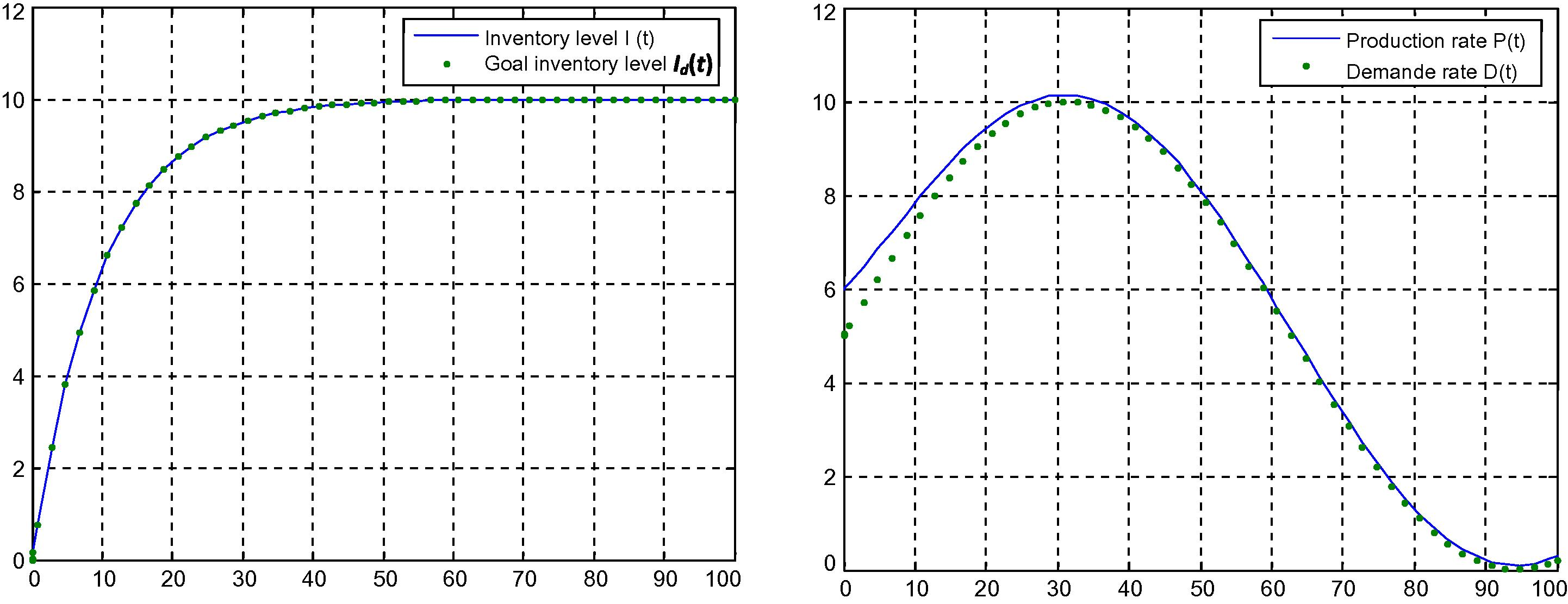
Simulation example: Let us assume, for example, that items in stock deteriorate at a rate of $\theta =0.01$ , so that

Close

Figure 1

Results of model reference control simulation.

Export to PPT

4 Model reference adaptive

A situation virtually always met in practice occurs when the deterioration rate is unknown. When the parameter θ is unknown, the control (3.1) cannot be implemented. Therefore, instead of (3.1), we propose the control

4.2

4.2 Stability analysis

The inventory system closed by the time varying feedback (4.1) can be represented by: $$\left\{\begin{array}{c}\dot{e}=-a_{d}e+\mathrm{\Delta }\ell u_d-\mathrm{\Delta }\mathit{kI}\text{,}\hfill \\ \mathrm{\Delta }\dot{k}={\gamma }_1\mathit{eI}\text{,}\hfill \\ \mathrm{\Delta }\dot{\ell }=-{\gamma }_2{\mathit{eu}}_d\text{.}\hfill \end{array}\right.$$ The above closed loop system can be written under matrix form: $\dot{x}=A(t\text{,}I\text{,}{u}_d)x(t)$ where $x={[\begin{array}{ccc}\hfill e\hfill & \hfill \mathrm{\Delta }k\hfill & \hfill \mathrm{\Delta }\ell \hfill \end{array}]}^T$ represents the state of the inventory system in closed loop and $A(t\text{,}I\text{,}{u}_d)=\left[\begin{array}{ccc}\hfill -a_d\hfill & \hfill -I\hfill & \hfill u_d\hfill \\ \hfill {\gamma }_{1}I\hfill & \hfill 0\hfill & \hfill 0\hfill \\ \hfill -{\gamma }_2{u}_d\hfill & \hfill 0\hfill & \hfill 0\hfill \end{array}\right]$ is the state matrix.

The Lyapunov function can be rewritten as: $V(e\text{,}\mathrm{\Delta }k\text{,}\mathrm{\Delta }\ell )=V(x)=\frac{e^2}{2}+\frac{\mathrm{\Delta }{k}^2}{2{\gamma }_1}+\frac{\mathrm{\Delta }{\ell }^2}{2{\gamma }_2}=\frac{1}{2}{x}^T\Gamma x>0$ . Since the matrix $\Gamma =\left[\begin{array}{ccc}\hfill 1\hfill & \hfill 0\hfill & \hfill 0\hfill \\ \hfill 0\hfill & \hfill \frac{1}{{\gamma }_1}\hfill & \hfill 0\hfill \\ \hfill 0\hfill & \hfill 0\hfill & \hfill \frac{1}{{\gamma }_2}\hfill \end{array}\right]$ is positive definite, that is, $V(x)>0$ in ${\mathfrak{R}}^3-\{\underline{0}\}$ where $\underline{0}={[\begin{array}{ccc}\hfill 0\hfill & \hfill 0\hfill & \hfill 0\hfill \end{array}]}^T$ is the equilibrium point or the origin of the closed loop system. We have $\dot{V}(x)=-a_{d}e⩽0$ .

Note that:

• When $e\ne 0$ , $\dot{V}<0$ , the state $x(t)$ converges toward the equilibrium point provided the tracking error $e\ne 0$ , until the state reaches the origin, in which case $e=0$ , $\mathrm{\Delta }k=0$ , i.e., $k(t)=k^{\ast }$ and $\mathrm{\Delta }\ell =0$ , i.e., $\ell ={\ell }^{\ast }$ .

• When $e=0$ before x(t) reaches the equilibrium point, $\dot{V}=0$ and according to the theorem given above, x(t) converges to x₀, where $x_0={[\begin{array}{ccc}\hfill 0\hfill & \hfill \overline{k}\hfill & \hfill \overline{\ell }\hfill \end{array}]}^T$ , where $\overline{k}$ and $\overline{\ell }$ are constants. Thus, we have the tracking error $e=0$ , $I(t)=I_d$ , $\mathrm{\Delta }k=\overline{k}$ , i.e., $k(t)=k^{\ast }+\overline{k}$ and $\mathrm{\Delta }\ell =\overline{\ell }$ , i.e., $\ell (t)={\ell }^{\ast }+\overline{\ell }$ .

This shows that our system is stable and not asymptotically stable. Although in control theory, it is usually preferable to have an asymptotic stability $(x(t)\to \underline{0})$ instead of stability, in our case, stability $(e\to 0)$ is sufficient since the tracking performance is achieved $(I(t)\to I_d)$ .

Implementation: The MRAC control law (4.1) and (4.8) is easily implemented. The adaptive gains γ₁ and γ₂ can be chosen to be any positive real numbers; see Sastry and Bodson (1989). It is to be noted however that these values affect the transient performance of the closed loop system: large γ₁, γ₂ lead to faster convergence. The initial values $k(0)\text{,}\ell (0)$ are chosen to be a priori guesses of the unknown parameters k and $\ell$ , respectively. Small initial parameter error usually leads to better transient behavior. The reference model and input u_d are designed so that I_d describes the optimal trajectory to be followed by the state equation.

Simulation example: Consider the data of the previous section example, except for the deterioration rate θ that is supposed to be unknown now. We also take $$I_d=\left\{\begin{array}{cc}10\text{,}\hfill & 0⩽t<100\text{,}\hfill \\ 5\text{,}\hfill & 100⩽t⩽200\text{,}\hfill \end{array}\right.\text{and}{u}_d=\left\{\begin{array}{cc}1\text{,}\hfill & 0⩽t<100\text{,}\hfill \\ 0.5\text{,}\hfill & 100⩽t⩽200\text{.}\hfill \end{array}\right.$$ And ${\gamma }_1={\gamma }_2=0.2$ . 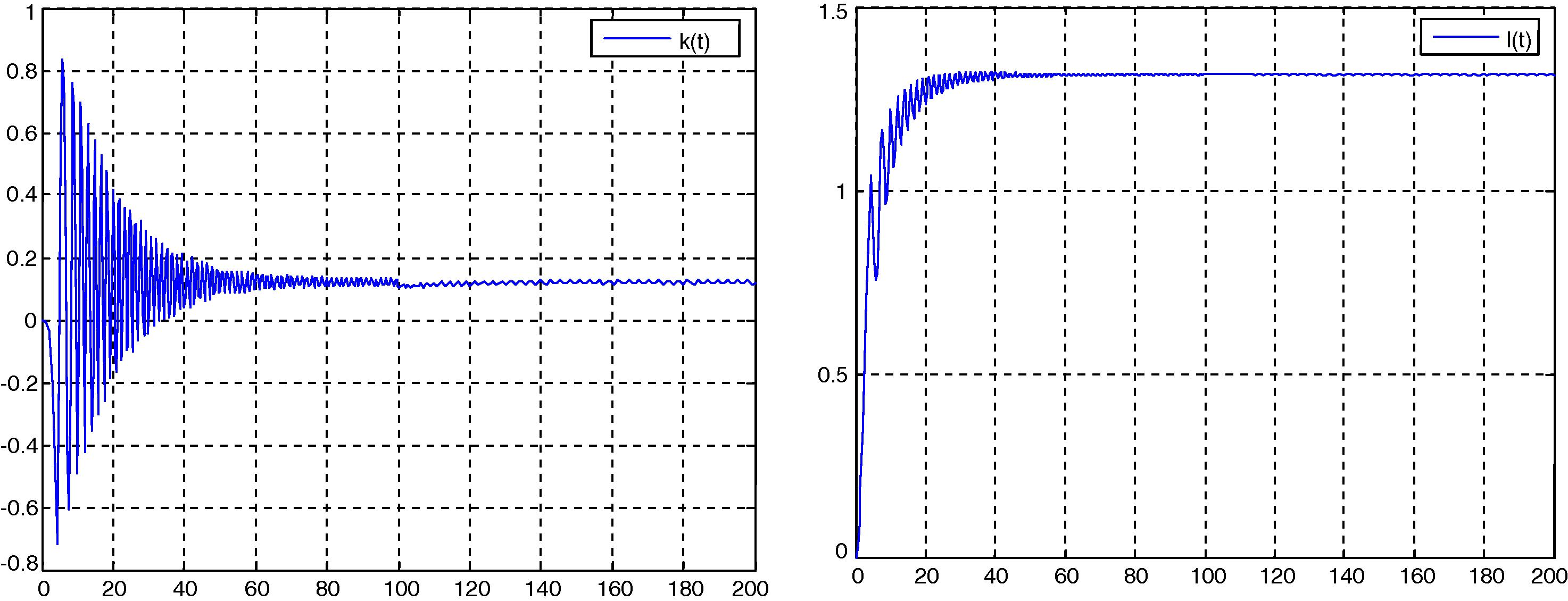A simulation was conducted for 200 units of time. First we show in Fig. 2 the convergence of k(t) to $\overline{k}$ (left) and $\ell (t)$ to $\overline{\ell }$ . Note that these results have been expected in the stability analysis.

Close

Figure 2

Convergence results of model reference adaptive control simulation.

Export to PPT

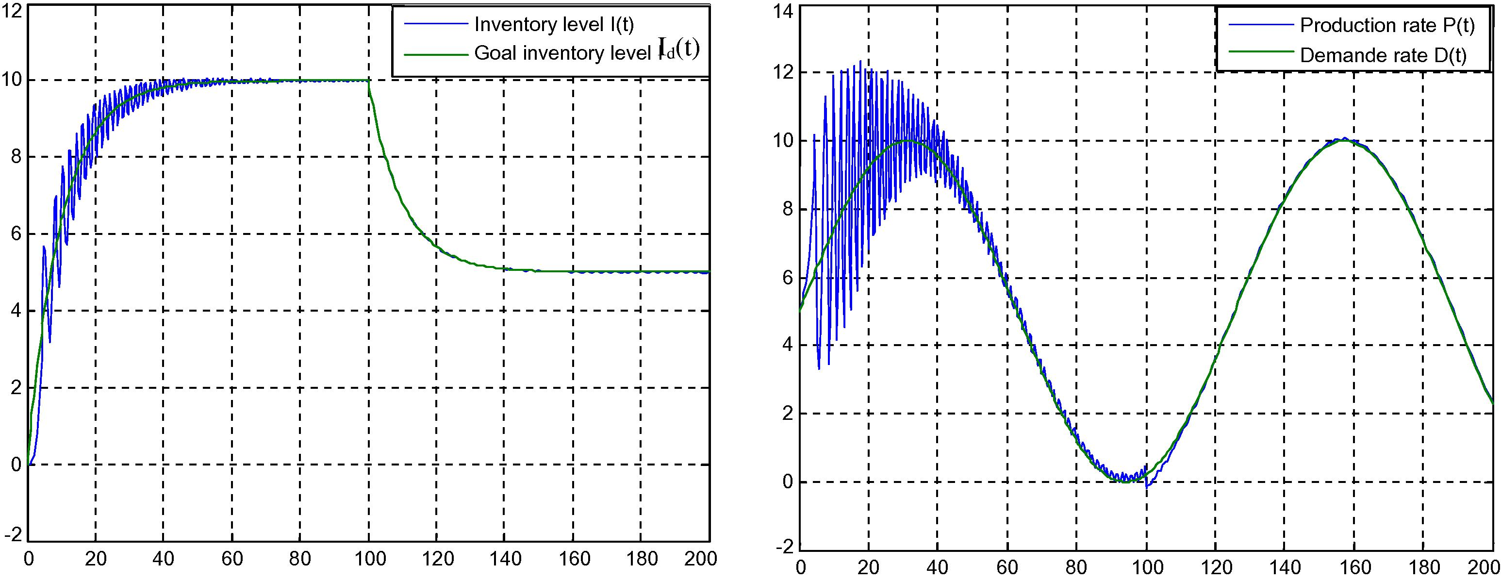
Fig. 3 shows the variations of the inventory level I(t) and the inventory goal level I_d (left) and the variations of the production rate P(t) and demand rate D(t) (right). It is depicted that after transient time, the inventory level I(t) tracks perfectly the inventory goal level $I_d(t)$ .

Close

Figure 3

Variations results of model reference adaptive control simulation.

Export to PPT

5 Conclusion

We have shown in this paper how to use an optimal control technique known as ‘Model reference adaptive control with feedback’ to solve a production-inventory planning problem. Simulations have been conducted to validate the results obtained. As a future research direction, we suggest the use of this technique on other inventory models, particularly those involving more than one differential equation, and on problems from other fields, such as economics, finance, etc.

References

- Recent trends in modeling of deteriorating inventory. European Journal of Operational Research. 2001;134:1-16.
- [Google Scholar]
- Predictive control of periodic-review production inventory systems with deteriorating items. TOP. 2004;12(1):193-208.
- Receding horizon control of a hybrid production system with deteriorating items. Nonlinear Analysis: Special Series on Hybrid Systems and Applications. 2005;63:405-422.
- Self-tuning optimal control of periodic-review production inventory systems with deteriorating items. Advanced Modeling and Optimization. 2007;9(1):91-104.
- Nonlinear Systems (third ed.). New Jersey: Prentice-Hall; 2002.
- Adaptive Control: Stability, Convergence, and Robustness. Englewood: Prentice-Hall; 1989.
- Optimal Control Theory: Applications to Management Science and Economics (second ed.). Dordrecht: Kluwer Academic Publishers; 2000.