The Nyström method for hybrid fuzzy differential equation IVPs

Omid Solaymani Fard; Tayebeh AliAbdoli Bidgoli

doi:10.1016/j.jksus.2010.07.020

View/Download PDF

Buy Reprints

PDF

Translate this page into:

ORIGINAL ARTICLE

23 (

); 371-379

doi:

10.1016/j.jksus.2010.07.020

The Nyström method for hybrid fuzzy differential equation IVPs

Omid Solaymani Fard^*, Tayebeh AliAbdoli Bidgoli

School of Mathematics and Computer Science, Damghan University, Damghan, Iran

*Corresponding author. Tel.: +98 5251253 omidsfard@gmail.com (Omid Solaymani Fard)

Received: 2010-6-25, Accepted: 2010-7-18, Published: 2010-10-01

Disclaimer:
This article was originally published by Elsevier and was migrated to Scientific Scholar after the change of Publisher.

Available online 21 July 2010

Peer-review under responsibility of King Saud University.

Abstract

In this paper, the Nyström method is developed to approximate the solutions for hybrid fuzzy differential equation initial value problems (IVPs) using the Seikkala derivative. A proof of convergence of this method is also discussed in detail. The accuracy and efficiency of the proposed method are demonstrated by applying it to two different numerical experiments.

Keywords

Hybrid systems

Fuzzy differential equations

Fuzzy interpolation

Fuzzy polynomials

Seikkala derivative

Nyström method

Show Related Articles from PubMed

1 Introduction

Fuzzy differential equation (FDE) models play a prominent role in a range of application areas, including papulation models (Guo and Li, 2003; Guo et al., 2003), civil engineering (Oberguggenberger and Pittschmann, 1999), particle systems (El Naschie, 2004a,b, 2005 ), medicine (Abbod et al., 2001; Barro and Marn, 2002; Helgason and Jobe, 1998; Nieto and Torres, 2003 ), bioinformatics and computational biology (Bandyopadhyay, 2005; Casasnovas and Rossell, 2005; Chang and Halgamuge, 2002 ). Particularly, the use of hybrid fuzzy differential equations (HFDEs) is a natural way to model control systems with embedded uncertainty (containing fuzzy valued functions) that are capable of controlling complex systems which have discrete event dynamics as well as continuous time dynamics.

In recent years, many works have been performed by several authors in numerical solutions of fuzzy differential equations (Fard, 2009a,b; Fard et al., 2009, 2010; Fard and Kamyad, 2010; Friedman et al., 1999; Hullermeier, 1999 ). Furthermore, there are some numerical techniques to solve hybrid fuzzy differential equations, for example, Pederson and Sambandham (2007, 2008) have investigated the numerical solution of HFDEs by using the Euler and Runge–Kutta methods, respectively, and Prakash and Kalaiselvi (2009) have studied the predictor–corrector method for hybrid fuzzy differential equations.

In this study, we develop numerical methods for hybrid fuzzy differential equations by an application of the Nyström method (Khastan and Ivaz, 2009). This paper is organized as follows: in Section 2, we provide some background on ordinary differential equations, fuzzy numbers and fuzzy differential equations. Section 3 contains a brief review of the hybrid fuzzy differential equation IVPs. In Sections 4 and 5, the Nyström method for hybrid fuzzy differential equations, a convergence theorem are discussed. Finally in Section 6, we present two numerical examples based on examples in Pederson and Sambandham (2007, 2008) to illustrate the theory.

2 Preliminaries

2.1

2.1 Notations and definitions

Definition 2.1

[Khastan and Ivaz (2009)] Consider the initial value problem

(1)

y^{'} (t) = f (t, y (t)), y (0) = y_{0},

where

f : [a, b] \times R^{n} \to R^{n}

. A m-step method for solving Eq. (1) is one whose difference equation for finding

y_{i + 1}

as approximation

y (t_{i + 1})

at the mesh point

t_{i + 1}

can be represented by the following equation:

(2)

y_{i + 1} = \sum_{j = 0}^{m - 1} a_{m - j - 1} y_{i - j} + h \sum_{j = 0}^{m - 1} b_{m - j} f (t_{i - j + 1}, y_{i - j + 1})

for

i = m - 1, m, \dots, N - 1

, such that

a = t_{0} ⩽ t_{1} ⩽ \dots ⩽ t_{N} = b

h = \frac{b - a}{N} = t_{i + 1} - t_{i}

and

a_{0}, a_{1}, \dots, a_{m - 1}

b_{0}, b_{1}, \dots, b_{m}

are constant with the starting values

y_{0} = α_{0}, y_{1} = α_{2}, \dots, y_{m - 1} = α_{m - 1}

When $b_{m} = 0$ , the method is known as explicit, since Eq. (2) gives $y_{i + 1}$ explicit in terms of previously determined values. Also, when $b_{m} \neq 0$ , the method is known as implicit, since $y_{i + 1}$ occurs on both sides of Eq. (2) and is specified only implicitly.

A especial case of multistep method is Nyström's methods (Henrici, 1962). Here, we set

(3)

y_{i + 1} = y_{i - 1} + h \sum_{m = 0}^{q} κ_{m} \nabla^{m} f (t_{i}, y_{i}), q = 0, 1, 2, \dots,

where the constants

κ_{m} = (- 1)^{m} \int_{- 1}^{1} (\begin{matrix} - s \\ m \end{matrix}) ds

are independent of f,

t = t_{0} + sh

\nabla f (t_{i}, y_{i})

is the first backward difference of the

f (t, y (t))

at the point of

t = t_{i}

and higher backward differences are defined by

\nabla^{k} f (t_{i}, y_{i}) = \nabla (\nabla^{k - 1} f (t_{i}, y_{i}))

. The special case

q = 0

of Nyström method is known as the midpoint rule:

y_{i + 1} = y_{i - 1} + 2 hf (t_{i}, y_{i}) .

Definition 2.2

(Henrici, 1962) Associated with the difference equation $\{\begin{matrix} y_{i + 1} = a_{m - 1} y_{i} + a_{m - 2} y_{i - 1} + \dots + a_{0} y_{i + 1 - m} \\ + hF (t_{i}, h, y_{i + 1}, y_{i}, \dots, y_{i + 1 - m}), \\ y_{0} = α_{0}, y_{1} = α_{1}, y_{2} = α_{2}, \dots, y_{m - 1} = α_{m - 1} \end{matrix}$ the following, called the characteristic polynomial of the method is $p (λ) = λ^{m} - a_{m - 1} λ^{m - 1} - a_{m - 2} λ^{m - 2} - \dots - a_{1} λ - a_{0} .$

If $| λ_{i} | ⩽ 1$ for each $i = 1, 2, \dots, m$ and all roots with absolute value 1 are simple roots, then the difference method is side to satisfy the root condition.

Theorem 2.3

A multistep method of the form (2) is stable if and only if satisfies the root condition.

Proof

See Isaacson and Keller (1966). □

Definition 2.4

A fuzzy number u is a fuzzy subset of the real line with a normal, convex and upper semicontinuous membership function of bounded support. The family of fuzzy numbers will be denoted by E. An arbitrary fuzzy number is represented by an ordered pair of functions $(\underline{u} (α), \bar{u} (α)), 0 ⩽ α ⩽ 1$ that, satisfies the following requirements:

–

$\underline{u} (α)$ is a bounded left continuous nondecreasing function over $[0, 1]$ , with respect to any $α$ .
–

$\bar{u} (α)$ is a bounded left continuous nonincreasing function over $[0, 1]$ , with respect to any $α$ .
–

$\underline{u} (α) ⩽ \bar{u} (α), 0 ⩽ α ⩽ 1$ .

Then, the $α$ -level set $[v]^{α} = {s | v (s) ⩾ 0}$ is a closed bounded interval, denoted $[v]^{α} = [{\underline{v}}^{α}, {\bar{v}}^{α}] .$

Definition 2.5

A triangular fuzzy number is a fuzzy set u in E that is characterized by an ordered triple $(u_{l}, u_{c}, u_{r}) \in R^{3}$ with $u_{l} ⩽ u_{c} ⩽ u_{r}$ such that $[u]^{0} = [u_{l}; u_{r}]$ and $[u]^{1} = {u_{c}}$ .

The $α$ -level set of a triangular fuzzy number u is given by

(4)

[u]^{α} = [u_{c} - (1 - α) (u_{c} - u_{l}), u_{c} + (1 - α) (u_{r} - u_{c})]

for any

α \in I = [0, 1]

Definition 2.6

Definition 2.6 Dubois and Prade, 2000

Let $A, B$ two nonempty bounded subsets of $R$ . The Hausdorff distance between A and B is $d_{H} (A, B) = \max [\sup_{a \in A} \inf_{b \in B} | a - b |, \sup_{b \in B} \inf_{a \in A} | a - b |] .$

The supremum metric D on E is as follows: $D (u, v) = \sup {d_{H} ([u]^{α}, [v]^{α}) : α \in I} .$

With the supremum metric, the space $(E, D)$ is a complete metric space.

Definition 2.7

Definition 2.7 Dubois and Prade, 2000

A fuzzy set-valued mapping $F : T \to E$ is continuous at $t_{0} \in T$ if for every $ε > 0$ there exists a $δ = δ (t_{0}, ε) > 0$ such that $D (F (t), F (t_{0})) < ε$ , for all $t \in T$ with $‖ t - t_{0} ‖ < δ$ .

Definition 2.8

Definition 2.8 Dubois and Prade, 2000

A mapping $F : T \to E$ is Hukuhara differentiable at $t_{0} \in T \subseteq R$ if for some $h_{0} > 0$ , the Hukuhara differences $F (t_{0} + Δ t) -_{h} F (t_{0})$ and $F (t_{0}) -_{h} F (t_{0} - Δ t)$ exist in E, for all $0 < Δ t < h_{0}$ and if there exists an $F^{'} (t_{0}) \in E$ such that $\lim_{Δ t \to 0} D (\frac{F (t_{0} + Δ t) -_{h} F (t_{0})}{Δ t} - F^{'} (t_{0})) = 0$ and $\lim_{Δ t \to 0} D (\frac{F (t_{0}) -_{h} F (t_{0} - Δ t)}{Δ t} - F^{'} (t_{0})) = 0 .$

The fuzzy set $F' (t_{0})$ is called the Hukuhara derivative of F at $t_{0}$ .

Definition 2.9

Definition 2.9 Dubois and Prade, 2000

The fuzzy integral $\int_{a}^{b} y (t) dt, 0 ⩽ a ⩽ b ⩽ 1,$ is defined by ${[\int_{a}^{b} y (t) dt]}^{α} = [\int_{a}^{b} {\underline{y}}^{α} dt, \int_{a}^{b} {\bar{y}}^{α} dt],$ provided the Lebesgue integrals on the right exist.

Remar 2.10

Remar 2.10 Kaleva, 1987

If $F : T \to E$ is Hukuhara differentiable and its Hukuhara derivative $F^{'}$ is integrable over $[0, 1],$ then $F (t) = F (t_{0}) + \int_{t_{0}}^{t} F^{'} (s) ds$ for all values of $t_{0}, t$ where $0 ⩽ t_{0} ⩽ t ⩽ 1$ .

Definition 2.11

Definition 2.11 Seikkala, 1987

Let I be a real interval. A mapping $y : I \to E$ is called a fuzzy process, and its $α$ -level set is denoted by $[y (t)]^{α} = [\underline{y} (t, α), \bar{y} (t, α)], t \in I, α \in (0, 1] .$

The Seikkala derivative $y^{'} (t)$ of a fuzzy process y is defined by $[y^{'} (t)]^{α} = [\underline{y^{'}} (t, α), \bar{y^{'}} (t, α)], t \in I, 0 < α ⩽ 1$ provided the is equation defines a fuzzy number $y^{'} (t) \in E$ .

Remar 2.12

Remar 2.12 Seikkala, 1987

If $y : I \to E$ is Seikkala differentiable and its Seikkala derivative $y^{'}$ is integrable over $[0, 1]$ , then $y (t) = y (t_{0}) + \int_{t_{0}}^{t} y^{'} (s) ds,$ for all values of $t_{0}, t$ where $t, t_{0} \in I$ .

2.2

2.2 Interpolation of fuzzy number

The problem of interpolation for fuzzy sets is as follows:

Suppose that at various time instant t information $f (t)$ is presented as fuzzy set. The aim is to approximate the function $f (t)$ , for all t in the domain of f. Let $t_{0} < t_{1} < \dots < t_{n}$ be $n + 1$ distinct points in R and let $u_{0}, u_{1}, \dots, u_{n}$ be $n + 1$ fuzzy sets in E. A fuzzy polynomial interpolation of the data is a fuzzy-value continuous function $f : R \to E$ satisfying:

$f (t_{i}) = u_{i}, i = 1, \dots, n$ .
If the data is crisp, then the interpolation f is a crisp polynomial.

A function f which fulfilling these condition may be constructed as follows. Let

C_{α}^{i} = [u_{i}]^{α}

for any

α \in [0, 1]

i = 0, 1, \dots, n .

For each

X = (x_{0}, x_{1}, \dots, x_{n}) \in R^{n + 1}

, the unique polynomial of

degree ⩽ n

denoted by

P_{X}

, such that

P_{X} (t_{i}) = x_{i}, i = 0, 1, \dots, n

and

P_{X} (t) = \sum_{i = 0}^{n} x_{i} (\prod_{i \neq j} \frac{t - t_{j}}{t_{i} - t_{j}}) .

Finally, for each

t \in R

and all

ξ \in R

is defined by

f (t) \in E

(f (t)) (ξ) = \sup {α \in [0, 1] : \exists X \in C_{α}^{0} \times C_{α}^{1} \times \dots \times C_{α}^{n} such that P_{X} (t) = ξ} .

The interpolation polynomial can be written level setwise as $[f (t)]^{α} = {y \in R : y = P_{X} (t), x_{i} \in [u_{i}]^{α}, i = 1, 2, \dots, n}, for 0 ⩽ α ⩽ 1$ when the data $u_{i}$ presents as triangular fuzzy numbers, values of the interpolation polynomial are also triangular fuzzy numbers. Then $f (t)$ has a particular simple form that is well suited to computation.

Theorem 2.13

Let $(t_{i}, u_{i}), i = 0, 1, 2, \dots, n$ be the observed data and suppose that each of $u_{i} = (u_{i}^{l}, u_{i}^{c}, u_{i}^{r})$ is a element of E. Then for each $t \in [t_{0}, t_{n}]$ , $f (t) = (f^{l} (t), f^{c} (t), f^{r} (t)) \in E$ , $\begin{matrix} f^{l} (t) = \sum_{l_{i} (t) ⩾ 0} l_{i} (t) u_{i}^{l} + \sum_{l_{i} (t) < 0} l_{i} (t) u_{i}^{r}, \\ f^{c} (t) = \sum_{i = 0}^{n} l_{i} (t) u_{i}^{c}, \\ f^{r} (t) = \sum_{l_{i} (t) ⩾ 0} l_{i} (t) u_{i}^{r} + \sum_{l_{i} (t) < 0} l_{i} (t) u_{i}^{l}, \end{matrix}$ where $l_{i} (t) = \prod_{j \neq i}^{n} \frac{t - t_{j}}{t_{i} - t_{j}}$ .

Proof

See Kaleva (1994). □

3 The hybrid fuzzy differential system

Consider the hybrid fuzzy differential system

(5)

\{\begin{matrix} x^{'} (t) = f (t, x (t), λ_{k} (x_{k})), t \in [t_{k}, t_{k + 1}], \\ x (t_{k}) = x_{k}, \end{matrix}

where

0 ⩽ t_{0} < t_{1} < \dots < t_{k} < \dots, t_{k} \to \infty, f \in C [R^{+} \times E \times E, E]

λ_{k} \in C [E, E]

Here, we assume that the existence and uniqueness of solution of the hybrid system hold on each $[t_{k}, t_{k + 1}]$ to be specific the system would look like: $x^{'} (t) = \{\begin{matrix} x_{0}^{'} (t) = f (t, x_{0} (t), λ_{0} (x_{0})), x (t_{0}) = x_{0}, t \in [t_{0}, t_{1}], \\ x_{1}^{'} (t) = f (t, x_{1} (t), λ_{1} (x_{1})), x (t_{1}) = x_{1}, t \in [t_{1}, t_{2}], \\ ⋮ \\ x_{k}^{'} (t) = f (t, x_{k} (t), λ_{k} (x_{k})), x (t_{k}) = x_{k}, t \in [t_{k}, t_{k + 1}], \\ ⋮ \end{matrix}$

By the solution of (5) we mean the following function: $x (t) = x (t, t_{0}, x_{0}) = \{\begin{matrix} x_{0} (t), t \in [t_{0}, t_{1}], \\ x_{1} (t), t \in [t_{1}, t_{2}], \\ ⋮ \\ x_{k} (t), t \in [t_{k}, t_{k + 1}], \\ ⋮ \end{matrix}$

We note that the solutions of (5) are piecewise differentiable in each interval for $t \in [t_{k}, t_{k + 1}]$ for a fixed $x_{k} \in E$ and $k = 0, 1, 2, \dots$ .

4 Nyström methods

In this section, for a hybrid fuzzy differential equation (5), we develop the Nyström method via an application of the Nyström method for fuzzy differential equations in (Khastan and Ivaz, 2009) when f and $λ_{k}$ in Eq. (5) can obtained via the Zadeh extension principle form $f \in C [R^{+} \times R \times R, R]$ and $λ_{k} \in C [R, R]$ . We assume that the existence and uniqueness of solutions of Eq. (5) hold for each $[t_{k}, t_{k + 1}]$ .

For a fixed r, we replace each interval $[t_{k}, t_{k + 1}]$ by a set of $N_{k} + 1$ discrete equally spaced grid points, $t_{k} = t_{k, 0} < t_{k, 1} < \dots < t_{k, N} = t_{k + 1}$ (including the endpoints) at which the exact solution $x (t)$ is approximated by some $y_{k} (t)$ .

Fix $k \in Z^{+}$ . The fuzzy initial value problem

(6)

\{\begin{matrix} x_{k}^{'} (t) = f (t, x_{k} (t), λ_{k} (x_{k})), t_{k} ⩽ t ⩽ t_{k + 1}, \\ x (t_{k}) = x_{k}, \end{matrix}

can be solved by Nyström method.

Let fuzzy initial values be $y_{k, i}, y_{k, i - 1}, \dots, y_{k, i - q}$ , i.e., $f (t_{k, i - j}, y_{k, i - j}, λ_{k} (y_{k})), j = 0, 1, \dots, q$ , which are triangular fuzzy numbers are shown by ${f^{l} (t_{k, i - j}, y_{k, i - j}, λ_{k} (y_{k})), f^{c} (t_{k, i - j}, y_{k, i - j}, λ_{k} (y_{k})), f^{r} (t_{k, i - j}, y_{k, i - j}, λ_{k} (y_{k}))}, j = 0, 1, \dots, q,$ also

(7)

y (t_{k, i + 1}) = y (t_{k, i - 1}) + \int_{t_{k, i - 1}}^{t_{k, i + 1}} f (t, y_{k} (t), λ_{k} (y_{k})) dt .

where

f (t, y_{k} (t), λ_{k} (y_{k})) = (f^{l} (t, y_{k} (t), λ_{k} (y_{k})), f^{c} (t, y_{k} (t), λ_{k} (y_{k})), f^{r} (t, y_{k} (t), λ_{k} (y_{k}))) .

By fuzzy interpolation, we have:

(8)

f_{x}^{l} (t, y_{k} (t), λ_{k} (y_{k})) = \sum_{\binom{j = 0}{l_{j} (t) ⩾ 0}}^{q} l_{j} (t) f^{l} (t_{k, i - j}, y (t_{k, i - j}), λ_{k} (y_{k})) + \sum_{\binom{j = 0}{l_{j} (t) < 0}}^{q} l_{j} (t) f^{r} (t_{k, i - j}, y (t_{k, i - j}), λ_{k} (y_{k})),

(9)

f_{x}^{c} (t, y_{k} (t), λ_{k} (y_{k})) = \sum_{j = 0}^{q} l_{j} (t) f^{c} (t_{k, i - j}, y (t_{k, i - j}), λ_{k} (y_{k})),

(10)

f_{x}^{r} (t, y_{k} (t), λ_{k} (y_{k})) = \sum_{\binom{j = 0}{l_{j} (t) ⩾ 0}}^{q} l_{j} (t) f^{r} (t_{k, i - j}, y (t_{k, i - j}), λ_{k} (y_{k})) + \sum_{\binom{j = 0}{l_{j} (t) < 0}}^{q} l_{j} (t) f^{l} (t_{k, i - j}, y (t_{k, i - j}), λ_{k} (y_{k})) .

where

f_{x} (t, y_{k} (t), λ_{k} (y_{k})) = (f_{x}^{l} (t, y_{k} (t), λ_{k} (y_{k})), f_{x}^{c} (t, y_{k} (t), λ_{k} (y_{k})), f_{x}^{r} (t, y_{k} (t), λ_{k} (y_{k})))

, interpolates

f (t, y_{k} (t), λ_{k} (y_{k}))

with the interpolation data given by the values

f (t_{k, i - j}, y_{k, i - j}, λ_{k} (y_{k})), j = 0, 1, \dots, q

and

l_{j} (t) = \prod_{\binom{l = 0}{l \neq j}}^{q} \frac{t - t_{k, i - l}}{t_{k, i - j} - t_{k, i - l}}

Regarding to the sign of $l_{j} (t)$ in the integrating interval $[t_{i - 1}, t_{i + 1}],$ we have from Eq. (7)

(11)

y (t_{k, i + 1}) = y (t_{k, i - 1}) + \int_{t_{k, i - 1}}^{t_{k, i}} f_{x} (t, y_{k} (t), λ_{k} (y_{k})) dt + \int_{t_{k, i}}^{t_{k, i + 1}} f_{x} (t, y_{k} (t), λ_{k} (y_{k})) dt .

The sign of $l_{j} (t)$ depends on q that is even or odd. We suppose q is even. Also for the q is odd, we can proceed similarly.

For $t_{k, i - 1} ⩽ t ⩽ t_{k, i}$ , by definition of $l_{j} (t)$ , we can write: $\begin{matrix} l_{r} (t) ⩾ 0 for r \in M = {0, 1, 3, \dots, q - 1} \\ l_{r} (t) < 0 for r \in N = {2, 4, \dots, q} \end{matrix}$ and for $t_{k, i} ⩽ t ⩽ t_{k, i + 1}$ : $\begin{matrix} l_{r} (t) ⩾ 0 for r \in M^{'} = {0, 2, 4, \dots, q} \\ l_{r} (t) < 0 for r \in N^{'} = {1, 3, \dots, q - 1} . \end{matrix}$

Thus, for $t_{k, i - 1} ⩽ t ⩽ t_{k, i}$ , we have:

(12)

\begin{matrix} f_{x}^{l} (t, y_{k} (t), λ_{k} (y_{k})) = \sum_{j \in M} l_{j} (t) f^{l} (t_{k, i - j}, y_{k, i - j}, λ_{k} (y_{k})) \\ + \sum_{j \in N} l_{j} (t) f^{r} (t_{k, i - j}, y_{k, i - j}, λ_{k} (y_{k})), \end{matrix}

(13)

f_{x}^{c} (t, y_{k} (t), λ_{k} (y_{k})) = \sum_{j \in M \cap N} l_{j} (t) f^{c} (t_{k, i - j}, y_{k, i - j}, λ_{k} (y_{k})),

(14)

\begin{matrix} f_{x}^{r} (t, y_{k} (t), λ_{k} (y_{k})) = \sum_{j \in M} l_{j} (t) f^{r} (t_{k, i - j}, y_{k, i - j}, λ_{k} (y_{k})) \\ + \sum_{j \in N} l_{j} (t) f^{l} (t_{k, i - j}, y_{k, i - j}, λ_{k} (y_{k})), \end{matrix}

and for

t_{k, i} ⩽ t ⩽ t_{k, i + 1}

(15)

\begin{matrix} f_{x}^{l} (t, y_{k} (t), λ_{k} (y_{k})) = \sum_{j \in M^{'}} l_{j} (t) f^{l} (t_{k, i - j}, y_{k, i - j}, λ_{k} (y_{k})) \\ + \sum_{j \in N^{'}} l_{j} (t) f^{r} (t_{k, i - j}, y_{k, i - j}, λ_{k} (y_{k})), \end{matrix}

(16)

f_{x}^{c} (t, y_{k} (t), λ_{k} (y_{k})) = \sum_{j \in M^{'} \cap N^{'}} l_{j} (t) f^{c} (t_{k, i - j}, y_{k, i - j}, λ_{k} (y_{k})),

(17)

\begin{matrix} f_{x}^{r} (t, y_{k} (t), λ_{k} (y_{k})) = \sum_{j \in M^{'}} l_{j} (t) f^{r} (t_{k, i - j}, y_{k, i - j}, λ_{k} (y_{k})) \\ + \sum_{j \in N^{'}} l_{j} (t) f^{l} (t_{k, i - j}, y_{k, i - j}, λ_{k} (y_{k})) . \end{matrix}

From (4) to (7) it follows that:

$y^{α} (t_{k, i + 1}) = [{\underline{y}}^{α} (t_{k, i + 1}), {\bar{y}}^{α} (t_{k, i + 1})]$ where

(18)

\begin{matrix} {\underline{y}}^{α} (t_{k, i + 1}) = {\underline{y}}^{α} (t_{k, i - 1}) + \int_{t_{k, i - 1}}^{t_{k, i + 1}} {α f^{c} (t, y_{k} (t), λ_{k} (y_{k})) \\ + (1 - α) f^{l} (t, y_{k} (t), λ_{k} (y_{k}))} dt, \end{matrix}

(19)

\begin{matrix} {\bar{y}}^{α} (t_{k, i + 1}) = {\bar{y}}^{α} (t_{k, i - 1}) + \int_{t_{k, i - 1}}^{t_{k, i + 1}} {α f^{c} (t, y_{k} (t), λ_{k} (y_{k})) \\ + (1 - α) f^{r} (t, y_{k} (t), λ_{k} (y_{k}))} dt . \end{matrix}

According to Eq. (11), if (12), (13), (15), (16) are situated in (18) and (13), (14), (16) and (17) in (19), we obtain ${\underline{y}}_{k, i + 1}^{α} = {\underline{y}}_{k, i - 1}^{α} + \int_{t_{k, i - 1}}^{t_{k, i}} \{α \sum_{j \in M \cap N} l_{j} (t) f^{c} (t_{k, i - j}, y_{k, i - j}, λ_{k} (y_{k})) + (1 - α) [\sum_{j \in M} l_{j} (t) f^{l} (t_{k, i - j}, y_{k, i - j}, λ_{k} (y_{k})) + \sum_{j \in N} l_{j} (t) f^{r} (t_{k, i - j}, y_{k, i - j}, λ_{k} (y_{k}))]\} dt + \int_{t_{k, i}}^{t_{k, i + 1}} \{α \sum_{j \in M^{'} \cap N^{'}} l_{j} (t) f^{c} (t_{k, i - j}, y_{k, i - j}, λ_{k} (y_{k})) + (1 - α) [\sum_{j \in M^{'}} l_{j} (t) f^{l} (t_{k, i - j}, y_{k, i - j}, λ_{k} (y_{k})) + \sum_{j \in N^{'}} l_{j} (t) f^{r} (t_{k, i - j}, y_{k, i - j}, λ_{k} (y_{k}))]\} dt = {\underline{y}}_{k, i - 1}^{α} + \sum_{j \in M} [α f^{c} (t_{k, i - j}, y_{k, i - j}, λ_{k} (y_{k})) + (1 - α) f^{l} (t_{k, i - j}, y_{k, i - j}, λ_{k} (y_{k}))] (\int_{t_{k, i - 1}}^{t_{k, i}} l_{j} (t) dt) + \sum_{j \in N} [α f^{c} (t_{k, i - j}, y_{k, i - j}, λ_{k} (y_{k})) + (1 - α) f^{r} (t_{k, i - j}, y_{k, i - j}, λ_{k} (y_{k}))] (\int_{t_{k, i - 1}}^{t_{k, i}} l_{j} (t) dt) + \sum_{j \in M^{'}} [α f^{c} (t_{k, i - j}, y_{k, i - j}, λ_{k} (y_{k})) + (1 - α) f^{l} (t_{k, i - j}, y_{k, i - j}, λ_{k} (y_{k}))] (\int_{t_{k, i}}^{t_{k, i + 1}} l_{j} (t) dt) + \sum_{j \in N^{'}} [α f^{c} (t_{k, i - j}, y_{k, i - j}, λ_{k} (y_{k})) + (1 - α) f^{r} (t_{k, i - j}, y_{k, i - j}, λ_{k} (y_{k}))] (\int_{t_{k, i}}^{t_{k, i + 1}} l_{j} (t) dt) .$

If we define $γ_{j} = \int_{t_{k, i - 1}}^{t_{k, i}} l_{j} (t) dt$ and $δ_{j} = \int_{t_{k, i}}^{t_{k, i + 1}} l_{j} (t) dt$ , thus from (4) we have

(20)

{\underline{y}}_{k, i + 1}^{α} = {\underline{y}}_{k, i - 1}^{α} + \sum_{j \in M} {\underline{f}}^{α} (t_{k, i - j}, y_{k, i - j}, λ_{k} (y_{k})) γ_{j} + \sum_{j \in N} {\bar{f}}^{α} (t_{k, i - j}, y_{k, i - j}, λ_{k} (y_{k})) γ_{j} + \sum_{j \in M^{'}} {\underline{f}}^{α} (t_{k, i - j}, y_{k, i - j}, λ_{k} (y_{k})) δ_{j} + \sum_{j \in N^{'}} {\bar{f}}^{α} (t_{k, i - j}, y_{k, i - j}, λ_{k} (y_{k})) δ_{j},

and we can deduce similarly

(21)

{\bar{y}}_{k, i + 1}^{α} = {\bar{y}}_{k, i - 1}^{α} + \sum_{j \in M} {\bar{f}}^{α} (t_{k, i - j}, y_{k, i - j}, λ_{k} (y_{k})) γ_{j} + \sum_{j \in N} {\underline{f}}^{α} (t_{k, i - j}, y_{k, i - j}, λ_{k} (y_{k})) γ_{j} + \sum_{j \in M^{'}} {\bar{f}}^{α} (t_{k, i - j}, y_{k, i - j}, λ_{k} (y_{k})) δ_{j} + \sum_{j \in N^{'}} {\underline{f}}^{α} (t_{k, i - j}, y_{k, i - j}, λ_{k} (y_{k})) δ_{j} .

Therefore, Nyström method is obtained as follows:

(22)

\{\begin{matrix} \begin{matrix} {\underline{y}}_{k, i + 1}^{α} = {\underline{y}}_{k, i - 1}^{α} + \sum_{j \in M} {\underline{f}}^{α} (t_{k, i - j}, y_{k, i - j}, λ_{k} (y_{k})) γ_{j} \\ + \sum_{j \in N} {\bar{f}}^{α} (t_{k, i - j}, y_{k, i - j}, λ_{k} (y_{k})) γ_{j} \\ + \sum_{j \in M^{'}} {\underline{f}}^{α} (t_{k, i - j}, y_{k, i - j}, λ_{k} (y_{k})) δ_{j} \\ + \sum_{j \in N^{'}} {\bar{f}}^{α} (t_{k, i - j}, y_{k, i - j}, λ_{k} (y_{k})) δ_{j}, \end{matrix} \\ \begin{matrix} {\bar{y}}_{k, i + 1}^{α} = {\bar{y}}_{k, i - 1}^{α} + \sum_{j \in M} {\bar{f}}^{α} (t_{k, i - j}, y_{k, i - j}, λ_{k} (y_{k})) γ_{j} \\ + \sum_{j \in N} {\underline{f}}^{α} (t_{k, i - j}, y_{k, i - j}, λ_{k} (y_{k})) γ_{j} \\ + \sum_{j \in M^{'}} {\bar{f}}^{α} (t_{k, i - j}, y_{k, i - j}, λ_{k} (y_{k})) δ_{j} \\ + \sum_{j \in N^{'}} {\underline{f}}^{α} (t_{k, i - j}, y_{k, i - j}, λ_{k} (y_{k})) δ_{j}, \end{matrix} \\ {\underline{y}}_{k, i - q}^{α} = α_{0}, {\underline{y}}_{k, i - q + 1}^{α} = α_{1}, \dots, {\underline{y}}_{k, i}^{α} = α_{q}, \\ {\bar{y}}_{k, i - q}^{α} = α_{q + 1}, {\bar{y}}_{k, i - q + 1}^{α} = α_{q + 2}, \dots, {\bar{y}}_{k, i}^{α} = α_{2 q + 1} . \end{matrix}

Worthy of note is the especial case $q = 0$ . Here $γ_{0} = h, δ_{0} = h$ and (22) becomes

(23)

\{\begin{matrix} {\underline{y}}_{k, i + 1}^{α} = {\underline{y}}_{k, i - 1}^{α} + 2 h {\underline{f}}^{α} (t_{k, i}, y_{k, i}, λ_{k} (y_{k})), \\ {\bar{y}}_{k, i + 1}^{α} = {\bar{y}}_{k, i - 1}^{α} + 2 h {\bar{f}}^{α} (t_{k, i}, y_{k, i}, λ_{k} (y_{k})), \\ {\underline{y}}_{k, i - 1}^{α} = α_{0}, {\underline{y}}_{k, i}^{α} = α_{1}, {\bar{y}}_{k, i - 1}^{α} = α_{2}, {\bar{y}}_{k, i}^{α} = α_{3} . \end{matrix}

This is the so-called Midpoint rule.

5 Convergence

By Theorem 5.2 in Kaleva (1987), we may replace (5) by an equivalent system:

(24)

\{\begin{matrix} {\underline{x}}^{'} (t) = \underline{f} (t, x, λ_{k} (x_{k})) = F_{k} (t, \underline{x}, \bar{x}), \underline{x} (t_{k}) = {\underline{x}}_{k}, \\ {\bar{x}}^{'} (t) = \bar{f} (t, x, λ_{k} (x_{k})) = G_{k} (t, \underline{x}, \bar{x}), \bar{x} (t_{k}) = {\bar{x}}_{k}, \end{matrix}

which possesses a unique solution

(\underline{x}, \bar{x})

which is a fuzzy function. That is for each t, the pair

[\underline{x} (t, r), \bar{x} (t, r)]

is a fuzzy number, where

\underline{x} (t, r), \bar{x} (t, r)

are respectively the solutions of the parametric form given by:

(25)

\{\begin{matrix} {\underline{x}}^{'} (t, r) = F_{k} (t, \underline{x} (t, r), \bar{x} (t, r)), \underline{x} (t_{k}, r) = {\underline{x}}_{k} (r), \\ {\bar{x}}^{'} (t, r) = G_{k} (t, \underline{x} (t, r), \bar{x} (t, r)), \bar{x} (t_{k}, r) = {\bar{x}}_{k} (r), \end{matrix}

for

r \in [0, 1]

For a fixed r, to integrate the system in (25) in $[t_{0}, t_{1}], [t_{1}, t_{2}], \dots, [t_{k}, t_{k + 1}], \dots$ , we replace each interval by a set of $N_{k} + 1$ discrete equally spaced grid points (including the end points) at which the exact solution $(\underline{x} (t, r), \bar{x} (t, r))$ is approximated by some $({\underline{y}}_{k} (t, r), {\bar{y}}_{k} (t, r))$ . For the chosen grid points on $[t_{k}, t_{k + 1}]$ at $t_{k, i} = t_{k} + {ih}_{k}, h_{k} = \frac{t_{k + 1} - t_{k}}{N_{k}}$ , $0 ⩽ n ⩽ N_{k}$ , let $({\underline{Y}}_{k} (t, r), {\bar{Y}}_{k} (t, r)) \equiv (\underline{x} (t, r), \bar{x} (t, r))$ . $({\underline{Y}}_{k} (t, r), {\bar{Y}}_{k} (t, r))$ and $({\underline{y}}_{k} (t, r), {\bar{y}}_{k} (t, r))$ may be denoted respectively by $({\underline{Y}}_{k, i} (r), {\bar{Y}}_{k, i} (r))$ and $({\underline{y}}_{k, i} (r), {\bar{y}}_{k, i} (r))$ . For example, the Midpoint rule approximations ${\underline{Y}}_{k} (t, r)$ and ${\bar{Y}}_{k} (t, r)$ , Eq. (23), can be written as:

(26)

\{\begin{matrix} {\underline{y}}_{k, i + 1} (r) = {\underline{y}}_{k, i - 1} + 2 h_{k} F_{k} [t_{i, k}, {\underline{y}}_{k, i} (r), {\bar{y}}_{k, i} (r)], \\ {\bar{y}}_{k, i + 1} (r) = {\bar{y}}_{k, i - 1} + 2 h_{k} G_{k} [t_{i, k}, {\underline{y}}_{k, i} (r), {\bar{y}}_{k, i} (r)], \end{matrix}

However, (26) we will use ${\underline{y}}_{0, j} = {\underline{α}}_{j}, {\bar{y}}_{0, j} = {\bar{α}}_{j}, j = 0, 1$ and ${\underline{y}}_{k, j} = {\underline{y}}_{k - 1, N_{k - 1} + j} (α), {\bar{y}}_{k, j} = {\bar{y}}_{k - 1, N_{k - 1} + j} (α), j = 0, 1$ if $k ⩾ 1$ . Then (26) represents an approximation of ${\underline{Y}}_{k} (t, r)$ , ${\bar{Y}}_{k} (t, r)$ for each of the intervals $t_{0} ⩽ t ⩽ t_{1}, t_{1} ⩽ t ⩽ t_{2}, \dots, t_{k} ⩽ t ⩽ t_{k + 1}, \dots$ .

For a prefixed k and $r \in [0, 1]$ , the proof of convergence of the approximations in (22), i.e. $\lim_{h_{0}, \dots, h_{k} \to 0} {\underline{y}}_{k, N_{k}} (r) = \underline{x} (t_{k + 1}, r) and \lim_{h_{0}, \dots, h_{k} \to 0} {\bar{y}}_{k, N_{k}} (r) = \bar{x} (t_{k + 1}, r),$ is a application of Theorem 4.2. in Khastan and Ivaz (2009) and Lemma 5.1 below. The convergence is pointwise in r for a fixed k.

In the following, we show the convergence of the Midpoint rule, i.e., the Nyström method with $q = 0$ . For the other values of q, the proof can be done similarly.

Lemma 5.1

Suppose $i \in Z^{+}$ , $ε_{i} > 0$ , $r \in [0, 1]$ , and $h_{i} < 1$ are fixed. Let ${z_{i, n} (r)}_{n = 0}^{N_{i}}$ be the Midpoint approximation with $N = N_{i}$ to the fuzzy IVP:

(27)

\{\begin{matrix} x^{'} (t) = f (t, x (t), λ_{i} (x_{i})), t \in [t_{i}, t_{i + 1}] \\ x (t_{i}) = x_{i}, \end{matrix}

{y_{i, n} (r)}_{n = 0}^{N_{i}}

denotes the result of (26) from some

y_{i, 0} (r)

, then there exists a

δ_{i} > 0

such that

| {\underline{z}}_{i, 0} (r) - {\underline{y}}_{i, 0} (r) | < δ_{i}, | {\bar{z}}_{i, 0} (r) - {\bar{y}}_{i, 0} (r) | < δ_{i}

implies

| {\underline{z}}_{i, N_{i}} (r) - {\underline{y}}_{i, N_{i}} (r) | < ε_{i}, | {\bar{z}}_{i, N_{i}} (r) - {\bar{y}}_{i, N_{i}} (r) | < ε_{i} .

Proof

Fix $i \in Z^{+}$ , $ε_{i} > 0$ , $r \in [0, 1]$ , and $h_{i} < 1$ . Let ${z_{i, n} (r)}_{n = 0}^{N_{i}}$ be the Nyström approximation with $N = N_{i}$ to the fuzzy IVP (27). Suppose ${y_{i, n} (r)}_{n = 0}^{N_{i}}$ denotes the result of (26) from some $y_{i, 0} (r)$ . By (26), for each $l = 0, \dots, N_{i} - 1$ ,

(28)

| {\underline{z}}_{i, l + 1} (r) - {\underline{y}}_{i, l + 1} (r) | = | {\underline{z}}_{i, l} (r) + 2 h_{i} F_{i} [t_{i, l}, {\underline{z}}_{i, l} (r), {\bar{z}}_{i, l} (r)] - {\underline{y}}_{i, l} (r) - 2 h_{i} F_{i} [t_{i, l}, {\underline{y}}_{i, l} (r), {\bar{y}}_{i, l} (r)] | ⩽ | {\underline{z}}_{i, l} (r) - {\underline{y}}_{i, l} (r) | + 2 h_{i} | F_{i} [t_{i, l}, {\underline{z}}_{i, l} (r), {\bar{z}}_{i, l} (r)] - F_{i} [t_{i, l}, {\underline{y}}_{i, l} (r), {\bar{y}}_{i, l} (r)] |,

and

(29)

| {\bar{z}}_{i, l + 1} (r) - {\bar{y}}_{i, l + 1} (r) | = | {\bar{z}}_{i, l} (r) + 2 h_{i} G_{i} [t_{i, l}, {\underline{z}}_{i, l} (r), {\bar{z}}_{i, l} (r)] - {\bar{y}}_{i, l} (r) - 2 h_{i} G_{i} [t_{i, l}, {\underline{y}}_{i, l} (r), {\bar{y}}_{i, l} (r)] | ⩽ | {\bar{z}}_{i, l} (r) - {\bar{y}}_{i, l} (r) | + 2 h_{i} | G_{i} [t_{i, l}, {\underline{z}}_{i, l} (r), {\bar{z}}_{i, l} (r)] - G_{i} [t_{i, l}, {\underline{y}}_{i, l} (r), {\bar{y}}_{i, l} (r)] | .

Let $α_{N_{i}} = ε_{i}$ . Since $F_{i}$ and $G_{i}$ are continuous, there exists a $η_{N_{i}} > 0$ such that $| {\underline{z}}_{i, N_{i} - 1} (r) - {\underline{y}}_{i, N_{i} - 1} (r) | < η_{N_{i}}$ and $| {\bar{z}}_{i, N_{i} - 1} (r) - {\bar{y}}_{i, N_{i} - 1} (r) | < η_{N_{i}}$ imply

(30)

\begin{matrix} | F_{i} [t_{i, N_{i} - 1}, {\underline{z}}_{i, N_{i} - 1} (r), {\bar{z}}_{i, N_{i} - 1} (r)] - F_{i} [t_{i, N_{i} - 1}, {\underline{y}}_{i, N_{i} - 1} (r), \\ {\bar{y}}_{i, N_{i} - 1} (r)] | < \frac{ε_{i}}{4} = \frac{α_{N_{i}}}{4}, \end{matrix}

(31)

\begin{matrix} | G_{i} [t_{i, N_{i} - 1}, {\underline{z}}_{i, N_{i} - 1} (r), {\bar{z}}_{i, N_{i} - 1} (r)] - G_{i} [t_{i, N_{i} - 1}, {\underline{y}}_{i, N_{i} - 1} (r), \\ {\bar{y}}_{i, N_{i} - 1} (r)] | < \frac{ε_{i}}{4} = \frac{α_{N_{i}}}{4} . \end{matrix}

Let $α_{N_{i} - 1} = \min {\frac{ε_{i}}{2}, \frac{η_{N_{i}}}{2}}$ . If $| {\underline{z}}_{i, N_{i} - 1} (r) - {\underline{y}}_{i, N_{i} - 1} (r) | ⩽ α_{N_{i} - 1}$ and $| {\bar{z}}_{i, N_{i} - 1} (r) - {\bar{y}}_{i, N_{i} - 1} (r) | ⩽ α_{N_{i} - 1}$ then by (28) and (29) with $l = N_{i} - 1$ and (2) and (31) we have

(32)

| {\underline{z}}_{i, N_{i}} (r) - {\underline{y}}_{i, N_{i}} (r) | ⩽ | {\underline{z}}_{i, N_{i} - 1} (r) - {\underline{y}}_{i, N_{i} - 1} (r) | + 2 h_{i} | F_{i} [t_{i, N_{i} - 1}, {\underline{z}}_{i, N_{i} - 1} (r), {\bar{z}}_{i, N_{i} - 1} (r)] - F_{i} [t_{i, N_{i} - 1}, {\underline{y}}_{i, N_{i} - 1} (r), {\bar{y}}_{i, N_{i} - 1} (r)] | < α_{N_{i} - 1} + 2 h_{i} \frac{ε_{i}}{4} < \frac{ε_{i}}{2} + h_{i} \frac{ε_{i}}{2} < ε_{i} .

(33)

| {\bar{z}}_{i, N_{i}} (r) - {\bar{y}}_{i, N_{i}} (r) | ⩽ | {\bar{z}}_{i, N_{i} - 1} (r) - {\bar{y}}_{i, N_{i} - 1} (r) | + 2 h_{i} | G_{i} [t_{i, N_{i} - 1}, {\underline{z}}_{i, N_{i} - 1} (r), {\bar{z}}_{i, N_{i} - 1} (r)] - G_{i} [t_{i, N_{i} - 1}, {\underline{y}}_{i, N_{i} - 1} (r), {\bar{y}}_{i, N_{i} - 1} (r)] | < α_{N_{i} - 1} + 2 h_{i} \frac{ε_{i}}{4} < \frac{ε_{i}}{2} + h_{i} \frac{ε_{i}}{2} < ε_{i} .

Continue inductively for each $j = 2, \dots, N_{i}$ as follows. Since $F_{i}$ and $G_{i}$ are continuous, there exists a $η_{N_{i} - (j - 1)} > 0$ such that $| {\underline{z}}_{i, N_{i} - j} (r) - {\underline{y}}_{i, N_{i} - j} (r) | < η_{N_{i} - (j - 1)}$ and $| {\bar{z}}_{i, N_{i} - j} (r) - {\bar{y}}_{i, N_{i} - j} (r) | < η_{N_{i} - (j - 1)}$ imply

(34)

| F_{i} [t_{i, N_{i} - j}, {\underline{z}}_{i, N_{i} - j} (r), {\bar{z}}_{i, N_{i} - j} (r)] - F_{i} [t_{i, N_{i} - j}, {\underline{y}}_{i, N_{i} - j} (r), {\bar{y}}_{i, N_{i} - j} (r)] | < \frac{α_{N_{i} - (j - 1)}}{4},

(35)

| G_{i} [t_{i, N_{i} - j}, {\underline{z}}_{i, N_{i} - j} (r), {\bar{z}}_{i, N_{i} - j} (r)] - G_{i} [t_{i, N_{i} - j}, {\underline{y}}_{i, N_{i} - j} (r), {\bar{y}}_{i, N_{i} - j} (r)] | < \frac{α_{N_{i} - (j - 1)}}{4},

where

\frac{α_{N_{i} - (j - 1)}}{4}

was define in the previous step.

Let $α_{N_{i} - j} = \min {\frac{α_{N_{i} - (j - 1)}}{2}, \frac{η_{N_{i} - (j - 1)}}{2}}$ . If $| {\underline{z}}_{i, N_{i} - j} (r) - {\underline{y}}_{i, N_{i} - j} (r) | < α_{N_{i} - j}$ and $| {\bar{z}}_{i, N_{i} - j} (r) - {\bar{y}}_{i, N_{i} - j} (r) | < α_{N_{i} - j}$ then by (28) and (29) with $l = N_{i} - j$ and (34) and (35) we have

(36)

| {\underline{z}}_{i, N_{i} - (j - 1)} (r) - {\underline{y}}_{i, N_{i} - (j - 1)} (r) | ⩽ | {\underline{z}}_{i, N_{i} - j} (r) - {\underline{y}}_{i, N_{i} - j} (r) | + 2 h_{i} | F_{i} [t_{i, N_{i} - j}, {\underline{z}}_{i, N_{i} - j}, {\bar{z}}_{i, N_{i} - j}] - F_{i} [t_{i, N_{i} - j}, {\underline{y}}_{i, N_{i} - j}, {\bar{y}}_{i, N_{i} - j}] | < \frac{α_{N_{i} - (j - 1)}}{2} + 2 h_{i} \frac{α_{N_{i} - (j - 1)}}{4} < α_{N_{i} - (j - 1)},

(37)

| {\bar{z}}_{i, N_{i} - (j - 1)} (r) - {\bar{y}}_{i, N_{i} - (j - 1)} (r) | ⩽ | {\bar{z}}_{i, N_{i} - j} (r) - {\bar{y}}_{i, N_{i} - j} (r) | + 2 h_{i} | G_{i} [t_{i, N_{i} - j}, {\underline{z}}_{i, N_{i} - j}, {\bar{z}}_{i, N_{i} - j}] - G_{i} [t_{i, N_{i} - j}, {\underline{y}}_{i, N_{i} - j}, {\bar{y}}_{i, N_{i} - j}] | < \frac{α_{N_{i} - (j - 1)}}{2} + 2 h_{i} \frac{α_{N_{i} - (j - 1)}}{4} < α_{N_{i} - (j - 1)} .

Then, for $j = N_{j}$ we see $| {\underline{z}}_{i, 0} (r) - {\underline{y}}_{i, 0} (r) | < α_{0}$ and $| {\bar{z}}_{i, 0} (r) - {\bar{y}}_{i, 0} (r) | < α_{0}$ imply $| {\underline{z}}_{i, 1} (r) - {\underline{y}}_{i, 1} (r) | < α_{1} and | {\bar{z}}_{i, 1} (r) - {\bar{y}}_{i, 1} (r) | < α_{1} .$

For $j = N_{i} - 1$ we see $| {\underline{z}}_{i, 1} (r) - {\underline{y}}_{i, 1} (r) | < α_{1}$ and $| {\bar{z}}_{i, 1} (r) - {\bar{y}}_{i, 1} (r) | < α_{1}$ imply $| {\underline{z}}_{i, 2} (r) - {\underline{y}}_{i, 2} (r) | < α_{2} and | {\bar{z}}_{i, 2} (r) - {\bar{y}}_{i, 2} (r) | < α_{2} .$

Continue decreasing to $j = 2$ to see $| {\underline{z}}_{i, N_{i} - 2} (r) - {\underline{y}}_{i, N_{i} - 2} (r) | < α_{N_{i} - 2}$ and $| {\bar{z}}_{i, N_{i} - 2} (r) - {\bar{y}}_{i, N_{i} - 2} (r) | < α_{N_{i} - 2}$ imply $| {\underline{z}}_{i, N_{i} - 1} (r) - {\underline{y}}_{i, N_{i} - 1} (r) | < α_{N_{i} - 1} and | {\bar{z}}_{i, N_{i} - 1} (r) - {\bar{y}}_{i, N_{i} - 1} (r) | < α_{N_{i} - 1} .$

But it was already shown in (32) and (33) that ${\underline{z}}_{i, N_{i} - 1} (r) - {\underline{y}}_{i, N_{i} - 1} (r) | < α_{N_{i} - 1}$ and $| {\bar{z}}_{i, N_{i} - 1} (r) - {\bar{y}}_{i, N_{i} - 1} (r) | < α_{N_{i} - 1}$ imply $| {\underline{z}}_{i, N_{i}} (r) - {\underline{y}}_{i, N_{i}} (r) | < ε_{i} and | {\bar{z}}_{i, N_{i}} (r) - {\bar{y}}_{i, N_{i}} (r) | < ε_{i} .$

This proves the lemma with $δ_{i} = α_{0}$ . □

Theorem 5.2

Consider the systems (24) and (26). For a fixed $k \in Z^{+}$ and $r \in [0, 1],$

(38)

\lim_{h_{0}, \dots, h_{k} \to 0} {\underline{y}}_{k, N_{k}} (r) = \underline{x} (t_{k + 1}, r),

(39)

\lim_{h_{0}, \dots, h_{k} \to 0} {\bar{y}}_{k, N_{k}} (r) = \bar{x} (t_{k + 1}, r) .

Proof

Fix $k \in Z^{+}$ and $r \in [0, 1] .$ Choose $ε > 0$ . For each $i = 0, \dots, k$ we will find a $δ_{i}^{*} > 0$ such that $h_{i} < δ_{i}^{*}$ implies $| \underline{x} (t_{k + 1}, r) - {\underline{y}}_{k, N_{k}} (r) | < ε and | \bar{x} (t_{k + 1}, r) - {\bar{y}}_{k, N_{k}} (r) | < ε,$ where the $h_{i}$ values are allowable by regular partition of the $[t_{i}, t_{i + 1}]$ ’s. By Theorem 4.2. in Khastan and Ivaz (2009), there exists a $δ_{k}^{*} > 0$ such that if $h_{k} < δ_{k}^{*}$ then $| {\underline{z}}_{k, N_{k}} (r) - \underline{x} (t_{k + 1}, r) | < \frac{ε}{2} and ‖ {\bar{z}}_{k, N_{k}} (r) - \bar{x} (t_{k + 1}, r) | < \frac{ε}{2} .$

We may assume $δ_{k}^{*} < 1$ . Then $h_{k} < 1$ . By Lemma 5.1 there exists a $δ_{k} > 0$ such that

(40)

| {\underline{z}}_{k, 0} (r) - {\underline{y}}_{k, 0} (r) | < δ_{k} | {\bar{z}}_{k, 0} (r) - {\bar{y}}_{k, 0} (r) | < δ_{k}

implies

| {\underline{z}}_{k, N_{k}} (r) - {\underline{y}}_{k, N_{k}} (r) | < \frac{ε}{2} and | {\bar{z}}_{k, N_{k}} (r) - {\bar{y}}_{k, N_{k}} (r) | < \frac{ε}{2} .

Therefore if $h_{i} < δ_{k}^{*}$ and (40) holds then

(41)

\begin{matrix} | \underline{x} (t_{k + 1}, r) - {\underline{y}}_{k, N_{k}} (r) | ⩽ | \underline{x} (t_{k + 1}, r) - {\underline{z}}_{k, N_{k}} (r) | + | {\underline{z}}_{k, N_{k}} (r) \\ - {\underline{y}}_{k, N_{k}} (r) | < \frac{ε}{2} + \frac{ε}{2} = ε, \end{matrix}

(42)

\begin{matrix} | \bar{x} (t_{k + 1}, r) - {\bar{y}}_{k, N_{k}} (r) | ⩽ | \bar{x} (t_{k + 1}, r) - {\bar{z}}_{k, N_{k}} (r) | + | {\bar{z}}_{k, N_{k}} (r) \\ - {\bar{y}}_{k, N_{k}} (r) | < \frac{ε}{2} + \frac{ε}{2} = ε . \end{matrix}

By Theorem 4.2. in Khastan and Ivaz (2009), there exists a $δ_{k - 1}^{*} > 0$ such that if $h_{k - 1} < δ_{k - 1}^{*}$ then $| {\underline{z}}_{k - 1, N_{k - 1}} (r) - \underline{x} (t_{k}, r) | < \frac{δ_{k}}{2} and | {\bar{z}}_{k - 1, N_{k - 1}} (r) - \bar{x} (t_{k}, r) | < \frac{δ_{k}}{2} .$

We may assume $δ_{k - 1}^{*} < 1$ . Then $h_{k - 1} < 1$ . By Lemma 5.1 there exists a $δ_{k - 1} > 0$ such that

(43)

| {\underline{z}}_{k - 1, 0} (r) - {\underline{y}}_{k - 1, 0} (r) | < δ_{k - 1}, | {\bar{z}}_{k - 1, 0} (r) - {\bar{y}}_{k - 1, 0} (r) | < δ_{k - 1}

implies

| {\underline{z}}_{k - 1, N_{k - 1}} (r) - {\underline{y}}_{k - 1, N_{k - 1}} (r) | < \frac{δ_{k}}{2}, and | {\bar{z}}_{k - 1, N_{k - 1}} (r) - {\bar{y}}_{k - 1, N_{k - 1}} (r) | < \frac{δ_{k}}{2} .

Therefore if $h_{k - 1} < δ_{k - 1}^{*}$ and (43) holds then

(44)

| \underline{x} (t_{k}, r) - {\underline{y}}_{k - 1, N_{k - 1}} (r) | ⩽ | \underline{x} (t_{k}, r) - {\underline{z}}_{k - 1, N_{k - 1}} (r) | + | {\underline{z}}_{k - 1, N_{k - 1}} (r) - {\underline{y}}_{k - 1, N_{k - 1}} (r) | < \frac{δ_{k}}{2} + \frac{δ_{k}}{2} = δ_{k},

(45)

| \bar{x} (t_{k}, r) - {\bar{y}}_{k - 1, N_{k - 1}} (r) | ⩽ | \bar{x} (t_{k}, r) - {\bar{z}}_{k - 1, N_{k - 1}} (r) | + | {\bar{z}}_{k - 1, N_{k - 1}} (r) - {\bar{y}}_{k - 1, N_{k - 1}} (r) | < \frac{δ_{k}}{2} + \frac{δ_{k}}{2} = δ_{k} .

Continue inductively for each $i = k - 2, \dots, 2, 1$ to find a $δ_{i}^{*} > 0$ such that if $h_{i} < δ_{i}^{*}$ then $| {\underline{z}}_{i, N_{i}} (r) - \underline{x} (t_{i + 1}, r) | < \frac{δ_{i + 1}}{2} and | {\bar{z}}_{i, N_{i}} (r) - \bar{x} (t_{i + 1}, r) | < \frac{δ_{i + 1}}{2} .$

We may assume each $δ_{i}^{*} < 1$ . Then each $h_{i} < 1$ . By Lemma 5.1 there exists a $δ_{i} > 0$ such that

(46)

| {\underline{z}}_{i, 0} (r) - {\underline{y}}_{i, 0} (r) | < δ_{i}, | {\bar{z}}_{i, 0} (r) - {\bar{y}}_{i, 0} (r) | < δ_{i}

implies

(47)

| {\underline{z}}_{i, N_{i}} (r) - {\underline{y}}_{i, N_{i}} (r) | < \frac{δ_{i + 1}}{2}, and | {\bar{z}}_{i, N_{i}} (r) - {\bar{y}}_{i, N_{i}} (r) | < \frac{δ_{i + 1}}{2} .

Therefore if $h_{i} < δ_{i}^{*}$ and (46) holds then $\begin{matrix} | \underline{x} (t_{i + 1}, r) - {\underline{y}}_{i, N_{i}} (r) | ⩽ | \underline{x} (t_{i + 1}, r) - {\underline{z}}_{i, N_{i}} (r) | + | {\underline{z}}_{i, N_{i}} (r) - {\underline{y}}_{i, N_{i}} (r) | \\ < \frac{δ_{i + 1}}{2} + \frac{δ_{i + 1}}{2} = δ_{i + 1}, \\ | \bar{x} (t_{i + 1}, r) - {\bar{y}}_{i, N_{i}} (r) | ⩽ | \bar{x} (t_{i + 1}, r) - {\bar{z}}_{i, N_{i}} (r) | + | {\bar{z}}_{i, N_{i}} (r) - {\bar{y}}_{i, N_{i}} (r) | \\ < \frac{δ_{i + 1}}{2} + \frac{δ_{i + 1}}{2} = δ_{i + 1} . \end{matrix}$

In particular, there exists a $δ_{1}^{*} > 0$ such that if $h_{1} < δ_{1}^{*}$ and (46) holds with $i = 1$ then $| \underline{x} (t_{2}, r) - {\underline{y}}_{1, N_{1}} (r) | < δ_{2} and | \bar{x} (t_{2}, r) - {\bar{y}}_{1, N_{1}} (r) | < δ_{2} .$

By Theorem 4.2. in Khastan and Ivaz (2009), we may choose $δ_{0}^{*}$ such that $h_{0} < δ_{0}^{*}$ implies

(48)

| \underline{x} (t_{1}, r) - {\underline{y}}_{0, N_{0}} (r) | < δ_{1} and | \bar{x} (t_{1}, r) - {\bar{y}}_{0, N_{0}} (r) | < δ_{1} .

Suppose for each $i = 0, \dots, k$ that $h_{i} < δ_{i}^{*}$ . Since (48) is the same as (46) with $i = 1,$ we obtain (47) with $i = 1$ . Since (47) with $i = 1$ implies (46) with $i = 2$ , we obtain (47) with $i = 2$ . Continue inductively to obtain (40) and (41), proving (38) and (39). □

6 Numerical illustration

To give a clear overview of our study and to illustrate the above discussed technique, we consider the following examples.

Example 6.1

Consider the following hybrid fuzzy IVP,

(49)

\{\begin{matrix} x^{'} (t) = x (t) + m (t) λ_{k} (x (t_{k})), t \in [t_{k}, t_{k} + 1], \\ t_{k} = k, k = 0, 1, 2, \dots \\ x (0) = [0.75, 1, 1.125], \\ x (0.1) = [0.75 e^{0.1}, e^{0.1}, 1.125 e^{0.1}], \end{matrix}

where

(50)

m (t) = \{\begin{matrix} 2 (t (\mod 1)), if t (\mod 1) ⩽ 0.5 \\ 2 (1 - t (\mod 1)), if t (\mod 1) > 0.5, \end{matrix}

and

(51)

λ_{k} (μ) = \{\begin{matrix} \hat{0}, if k = 0, \\ μ, if k \in {1, 2, \dots} . \end{matrix}

For the which $\hat{0} \in E$ define as $\hat{0} (x) = 1$ if $x = 0$ and $\hat{0} (x) = 0$ if $x \neq 0$ . The hybrid fuzzy initial value problem (49) is equivalent to the following system of fuzzy initial value problems: $\{\begin{matrix} x_{0}^{'} (t) = x_{0} (t), t \in [0, 1], \\ x (0) = [0.75 + 0.25 α, 1.125 - 0.125 α], \\ x (0.1) = [(0.75 + 0.25 α) e^{0.1}, (1.125 - 0.125 α) e^{0.1}], \\ x_{i}^{'} (t) = x_{i} (t) + m (t) x_{i} (t_{i}), t \in [t_{i}, t_{i + 1}], \\ x_{i} (t_{i}) = x_{i - 1} (t_{i}), x_{i} (t_{i - 1, N_{i}}) = x_{i - 1} (t_{i - 1, N_{i}}), i = 1, 2, 3, \dots \end{matrix}$

In (49), $x (t) + m (t) λ_{k} (x_{k} (t))$ is a continuous function of $t, x$ and $λ_{k} (x (t_{k}))$ . Therefore by Example 6.1 of Kaleva (1987), for each $k = 0, 1, 2, \dots,$ the fuzzy IVP

(52)

\{\begin{matrix} x^{'} (t) = x (t) + m (t) λ_{k} (x (t_{k})), t \in [t_{k}, t_{k + 1}], t_{k} = k, \\ x (t_{k}) = x_{t_{k}}, \end{matrix}

has a unique solution on

[t_{k}, t_{k + 1}]

. To numerically solve the hybrid fuzzy IVP (49) we will apply the Midpoint rule method for this hybrid fuzzy differential equations with

N = 10

. For

[0, 1]

, the exact solution of (49) satisfies

x (t) = [0.75 e^{t}, e^{t}, 1.125 e^{t}] .

For $[1, 1.5]$ , the exact solution of (49) satisfies $x (t) = x (1) (3 e^{t - 1} - 2 t) .$

For $[1.5, 2]$ , the exact solution of (49) satisfies $x (t) = x (1) (2 t - 2 + e^{t - 1.5} (3 \sqrt{e} - 4)) .$

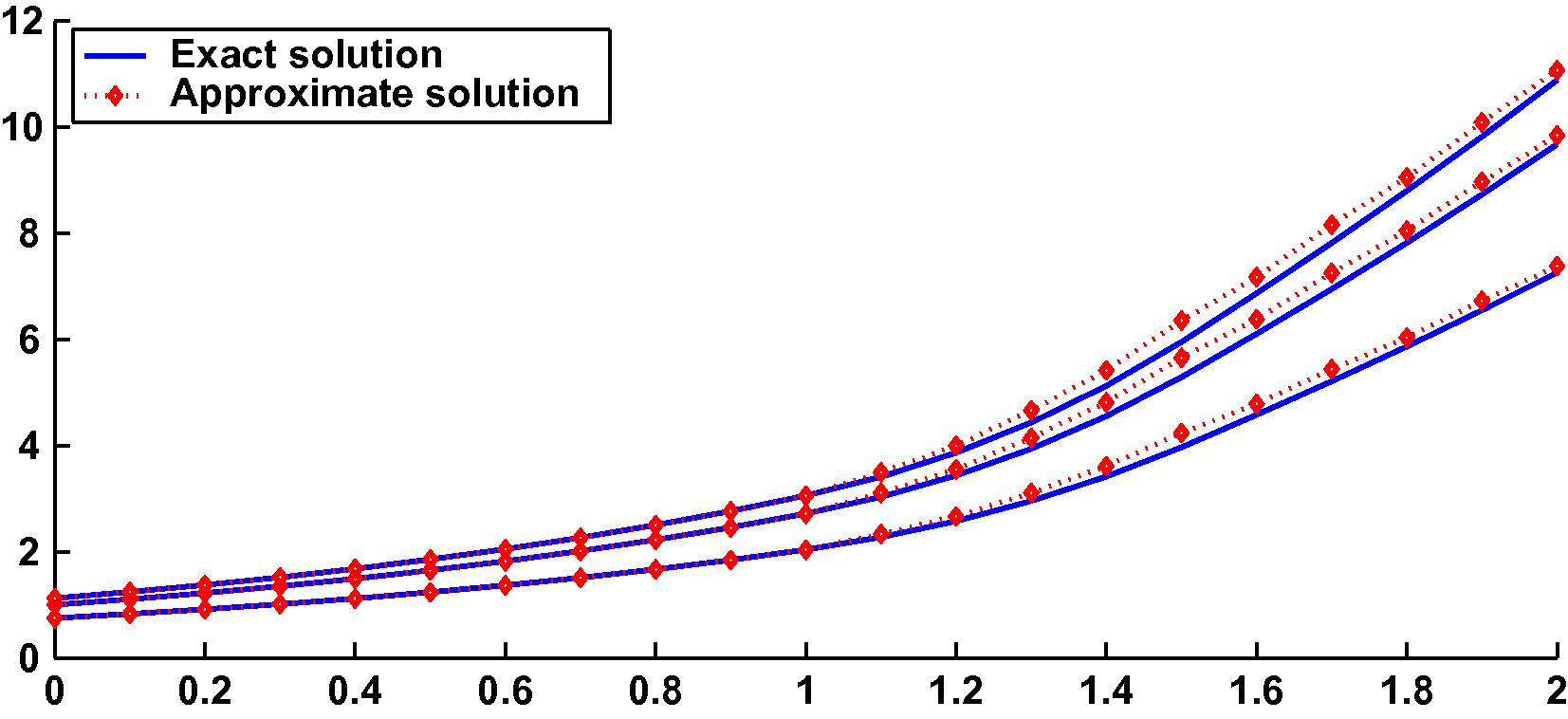
The comparison between the exact and numerical solutions on $[0, 2]$ is shown in Fig. 1.

Example 6.2

Consider the following hybrid fuzzy IVP,

(53)

\{\begin{matrix} x^{'} (t) = - x (t) + m (t) λ_{k} (x_{k})), t \in [t_{k}, t_{k + 1}], \\ t_{k} = k, k = 0, 1, 2, \dots, \\ x (0) = [0.75, 1, 1.125], \\ x (0.1) = [- 0.1875 e^{0.1} + 0.9375 e^{- 0.1}, e^{- 0.1}, 0.1875 e^{0.1} \\ + 0.9375 e^{- 0.1}], \end{matrix}

where

(54)

m (t) = | \sin (π t) |, k = 0, 1, 2, \dots,

and

(55)

λ_{k} (μ) = \{\begin{matrix} \hat{0}, if k = 0, \\ μ, if k \in {1, 2, \dots} . \end{matrix}

The hybrid fuzzy initial value problem (53) is equivalent to the following system:

(56)

\{\begin{matrix} x_{0}^{l'} (t) = - x_{0}^{r} (t), \\ x_{0}^{c'} (t) = - x_{0}^{c} (t), \\ x_{0}^{r'} (t) = - x_{0}^{l} (t), t \in [0, 1], \\ x (0) = [0.75, 1, 1.125], \\ x (0.1) = [- 0.1875 e^{0.1} + 0.9375 e^{- 0.1}, e^{- 0.1}, 0.1875 e^{0.1} \\ + 0.9375 e^{- 0.1}], \\ x_{i}^{l'} (t) = - x_{i}^{r} (t) + m (t) x_{i}^{l} (t_{i}), \\ x_{i}^{c'} (t) = - x_{i}^{c} (t) + m (t) x_{i}^{c} (t_{i}), \\ x_{i}^{r'} (t) = - x_{i}^{l} (t) + m (t) x_{i}^{r} (t_{i}), t \in [t_{i}, t_{i + 1}], \\ x_{i} (t_{i}) = x_{i - 1} (t_{i}), x_{i} (t_{i - 1, N_{i}}) = x_{i - 1} (t_{i - 1, N_{i}}), i = 1, 2, 3, \dots \end{matrix}

For [0, 1], the exact solution of Eq. (53) satisfies $x (t) = [- 0.1875 e^{t} + 0.9375 e^{- t}, e^{- t}, 0.1875 e^{t} + 0.9375 e^{- t}] .$

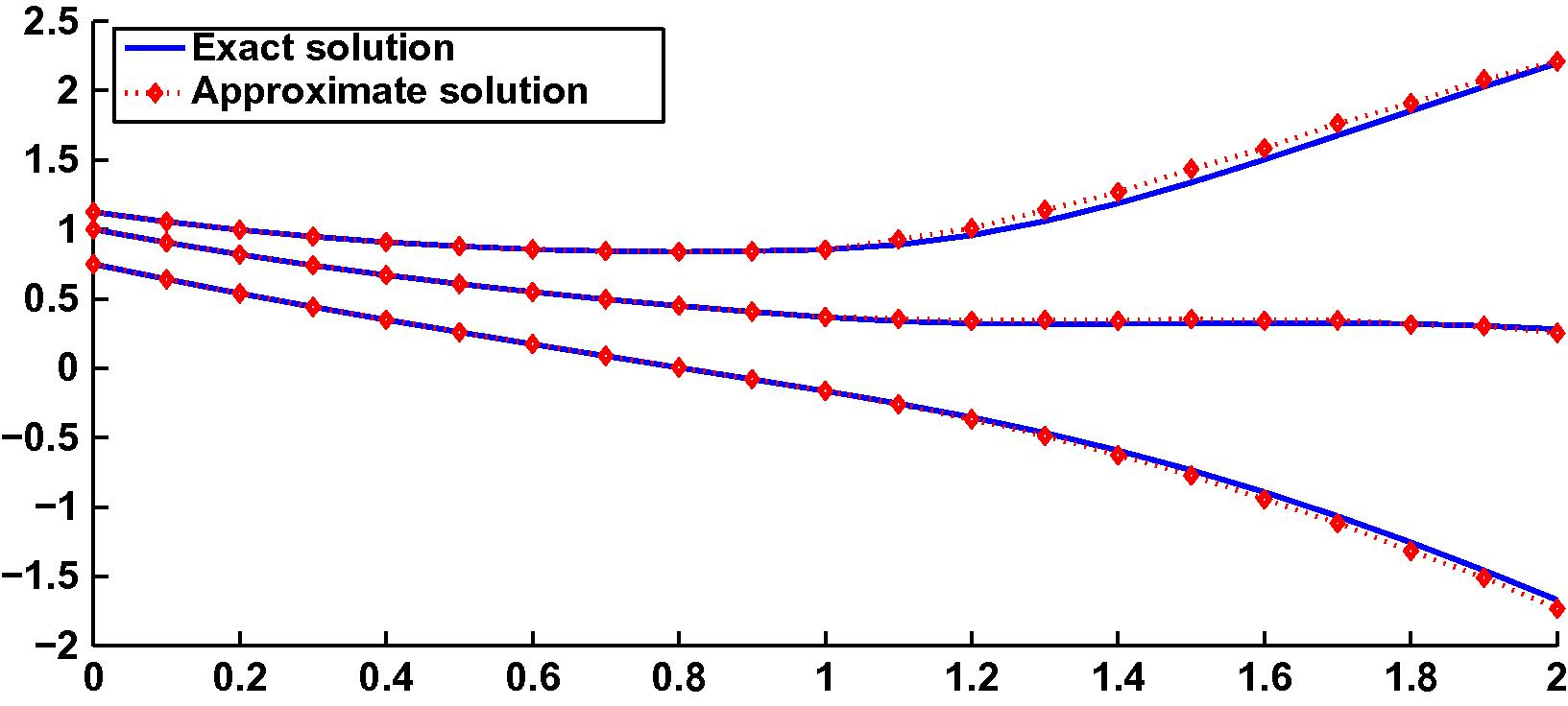
For [1, 2], the exact solution of Eq. (53) satisfies, $x (t)^{T} = (- 0.2417 e^{t} + 1.2085 e^{- t} - 0.0152 \cos (π t) π - 0.0786 \sin (π t) 1.2890 e^{- t} + 0.0338 \cos (π t) π - 0.0338 \sin (π t) 0.2417 e^{t} + 1.2085 e^{- t} + 0.0786 \cos (π t) π + 0.0152 \sin (π t))$

The comparison between the exact and numerical solutions on $[0, 2]$ is shown in Fig. 2.

References

Abbod M.F., Von Keyserlingk D.G., Linkens D.A., Mahfouf M., . Survey of utilisation of fuzzy technology in medicine and healthcare. Fuzzy Set Syst.. 2001;120:331-349.
[Google Scholar]
Bandyopadhyay S., . An efficient technique for superfamily classification of amino acid sequences: feature extraction, fuzzy clustering and prototype selection. Fuzzy Set Syst.. 2005;152:5-16.
[Google Scholar]
Barro S., Marn R., . Fuzzy Logic in Medicine. Heidelberg: Physica-Verlag; 2002.
Casasnovas J., Rossell F., . Averaging fuzzy biopolymers. Fuzzy Set Syst.. 2005;152:139-158.
[Google Scholar]
Chang B.C., Halgamuge S.K., . Protein motif extraction with neuro-fuzzy optimization. Bioinformatics. 2002;18:1084-1090.
[Google Scholar]
Dubois D., Prade H., . Fundamentals of Fuzzy Sets. USA: Kluwer Academic Publishers; 2000.
El Naschie M.S., . A review of E-infinite theory and the mass spectrum of high energy particle physics. Chaos Solitons Fract.. 2004;19:209-236.
[Google Scholar]
El Naschie M.S., . The concepts of E-infinite: an elementary introduction to the Cantorian-fractal theory of quantum physics. Chaos Solitons Fract.. 2004;22:495511.
[Google Scholar]
El Naschie M.S., . On a fuzzy Khler manifold which is consistent with the two slit experiment. Int. J. Nonlinear Sci. Numer. Simulat.. 2005;6:95-98.
[Google Scholar]
Fard O.S., . A numerical scheme for fuzzy cauchy problems. J. Uncertain Syst.. 2009;3:307-314.
[Google Scholar]
Fard O.S., . An iterative scheme for the solution of generalized system of linear fuzzy differential equations. World Appl. Sci. J.. 2009;7:1597-1604.
[Google Scholar]
Fard O.S., Hadi Z., Ghal-Eh N., Borzabadi A.H., . A note on iterative method for solving fuzzy initial value problems. J. Adv. Res. Sci. Comput.. 2009;1:22-33.
[Google Scholar]
Fard O.S., Bidgoli T.A., Borzabadi A.H., . Approximate-analytical approach to nonlinear FDEs under generalized differentiability. J. Adv. Res. Dyn. Control Syst.. 2010;2:56-74.
[Google Scholar]
Fard, O.S., Kamyad, A.V., 2010. Modified k-step method for solving fuzzy initial value problems. Iran. J. Fuzzy Syst.
Friedman M., Ma M., Kandel A., . Numerical solution of fuzzy differential and integral equations. Fuzzy Sets Syst.. 1999;106:35-48.
[Google Scholar]
Guo M., Li R., . Impulsive functional differential inclusions and fuzzy population models. Fuzzy Sets Syst.. 2003;138:601-615.
[Google Scholar]
Guo M., Xue X., Li R., . The oscillation of delay differential inclusions and fuzzy biodynamics models. Math. Comput. Model.. 2003;37:651-658.
[Google Scholar]
Helgason C.M., Jobe T.H., . The fuzzy cube and causal efficacy: representation of concomitant mechanisms in stroke. Neural Networks. 1998;11:549-555.
[Google Scholar]
Henrici P., . Discrete Variable Methods in Ordinary Differential Equations. John Wiley and Sons; 1962.
Hullermeier E., . Numerical methods for fuzzy initial value problems. Int. J. Uncertainty Fuzziness Knowledge-Based Syst.. 1999;7:439-461.
[Google Scholar]
Isaacson E., Keller H.B., . Analysis of Numerical Methods. New York: Wiley; 1966.
Kaleva O., . Fuzzy differential equations. Fuzzy Sets Syst.. 1987;24:301-317.
[Google Scholar]
Kaleva O., . Interpolation of fuzzy data. Fuzzy Sets Syst.. 1994;60:63-70.
[Google Scholar]
Khastan A., Ivaz K., . Numerical solution of fuzzy differential equations by Nyström method. Chaos, Solutions Fract.. 2009;41:859-868.
[Google Scholar]
Nieto J.J., Torres A., . Midpoints for fuzzy sets and their application in medicine. Artif. Intell. Med.. 2003;27:81-101.
[Google Scholar]
Oberguggenberger M., Pittschmann S., . Differential equations with fuzzy parameters. Math. Mod. Syst.. 1999;5:181-202.
[Google Scholar]
Pederson S., Sambandham M., . Numerical solution to hybrid fuzzy systems. Math. Comp. Model.. 2007;45:1133-1144.
[Google Scholar]
Pederson S., Sambandham M., . The Runge–Kutta method for hybrid fuzzy differential equations. Nonlinear Anal. Hybrid Syst.. 2008;2:626-634.
[Google Scholar]
Prakash P., Kalaiselvi V., . Numerical solution of hybrid fuzzy differential equations by predictor–corrector method. Int. J. Comp. Math.. 2009;86(1):121-134.
[Google Scholar]
Seikkala S., . On the fuzzy initial value problem. Fuzzy Sets Syst.. 1987;159:319-330.
[Google Scholar]