Tree-structured analysis of survival data and its application using SAS software

1 Introduction

The problems of modeling censored survival data have attracted much attention in the recent years. A very popular technique is the proportional hazard regression model, the most widely used model in the analysis of survival data, which is based on the fact that the logarithm of the hazard rate is a linear function of the covariates Cox (1972).

Proportional hazards model is used for investigating the effect on survival of covariates which are measured repeatedly over time. For a given time variable, the investigator records the times at which cohort members fail, the risk factors, and the potential confounding variables for each cohort member.

Survival distributions are considered at length by Lawless (2003). Multiple failure models have a long history in connection with competing risk or multiple decrements.

Important modern references include Hosmer et al. (2008), Lee and Wang (2003) and Kalbfleisch and Prentice (2002).

Tree-based methods for regression, and especially classification, are becoming popular alternatives to linear regression and linear discriminant analysis. Trees generally require fewer assumptions than classical methods and handle a wide variety of data structures. They provide another way of understanding the predictive structure of the data for both statisticians and the non statisticians. These methods (often called recursive partitioning) were originally developed by Morgan and Sonquist (1963); the classification and regression tree (CART) algorithm described in monograph by Breiman et al. (1984) greatly advanced the technology, and stimulated wide interest in tree-based techniques.

Breiman et al. (1984) have defined decision tree or automatic interaction detection (AID) as a method of partitioning a set of data, which is successively divided using explicative variables (risk factors, predictors,…) and referring to a dependent variable (response, outcome…).

Tree-structured analysis of survival data is considered as a powerful alternative (or complement) to traditional model building strategies such as Cox proportional hazards regression models using stepwise, or simply the forward method.

Several tree-based tools have been proposed for censored survival data (Ciampi et al., 1995; Davis and Anderson, 1989).

Decision trees as one of many data mining techniques has become a popular approach for segmentation, classification and prediction by applying a series of simple rules. The advantage that researchers have is that the results can be understood and explained easily, since it is expressed by a tree structured diagram as a final output. Some previous research work on decision tree dealt with survival data. LeBlanc and Crowley (1993) use log rank test, which is a non-parametric test. In this paper, we develop a recursive partition procedure based on semi-parametric regression (Cox regression or proportional hazards regression) for survival analysis using the forward technique.

One of the objectives of this paper is to explain how tree-structured analysis can be applied on survival data to split data into relatively homogenous subgroups. We consider an application using the real data (UIS data) [used by Hosmer et al. (2008)]. We use SAS (The Statistical Analysis System) as it provides an efficient way of computation.

Tree-structured survival analysis which is the object of this paper is defined as

• A way to select a split at every intermediate node. This is done by using Cox proportional hazard regression forward technique.

• A rule for determining when a node is terminal requires:

  • Size of the node is less than n₀ (pre assigned value) or

  • Statistical significance of a split.

2 Criteria used

Let an individual i, $i=1\text{,}\dots \text{,}N\text{,}$ be observed from time zero (i.e., date of starting investigation) to a failure or censoring time $t_i$ and let ${\delta }_i$ be the censoring indicators, taking value 1 if $t$ is failure time and 0 if it is a censoring time. Let x_ij $j=1\text{,}\dots \text{,}p$ be the jth question for individual i. Then the hazard function $h_i(t)$ for individual i, and jth question $x_{\mathit{ij}}$ for the data $(t_i\text{,}{\delta }_i\text{,}{x}_{\mathit{ij}})$ is $h_i(t)=h_0(t)\exp (b_j{x}_{\mathit{ij}})$ .

The quantity $h_0(t)$ is the baseline, and $b_j$ is unknown coefficient. We will obtain a sequence of nested sub-trees and calculate the incidence rate for each node. We assume that each explanatory variable $x_j$ is subdivided into two nodes with a risk denoted by $\pi (x_j)$ . The risk $\pi (.)$ is a result of rejecting for testing global null hypothesis: β = 0, which will be used in the algorithm to compare between partitions of nodes whose numbers of daughters (children, groups) are not usually equal; that is, the number of degree of freedom of $\pi (.)$ was different. A node will be split until it is not statistically significant or one of its children has too few observations.

3 UIS data

The data set consists of sample of UIS which stands for the University of Massachusetts Aids Research Unit (UMARU) IMPACT Study by Hosmer et al. (2008). It was a 5-year (1989–1994) collaborative research project comprised of two concurrent randomized trials of residential treatments for drug abuse. The purpose of that study was to compare treatment programs of different planned durations designed to reduce drug abuse and to prevent high-risk in HIV behavior.

The UIS sought to determine whether alternative residential treatment approaches vary in effectiveness and whether efficacy depends on planned program duration. The small subset of variables from the main study that we use in this paper is described in Table 1.

4 Data analysis

First, we deleted all the missing values. Then we recoded all variables to binary category using SAS. Note that we did not consider the LOT covariate since it is related to the outcome variable – time to drug use as measured from admission date (Hosmer et al., 2008). Table 2 presents the variables which will be used.

5 Applying cox proportional hazards model

We applied proportional hazards regression model given below: $$\log [h(t)/h_0(t)]={\beta }_1(\text{Race})+{\beta }_2(\text{Treat}){\beta }_3(\text{IVhx})+{\beta }_4(\text{Age})\text{.}$$

The estimates of the parameters of the model are given in Table 3.

We find the significant covariates are only race, treat, ivhx and age. Note that the covariate (beck) is significant if we consider the model which includes it alone, but in this model it is not significant because it is adjusted by other covariates.

Thus the model is: $$\log [h(t)/h_0(t)]=-0.26010(\text{Race})-0.21490(\text{Treat})+0.33840(\text{IVhx})+0.19633(\text{Age})\text{.}$$

Next, we applied the proportional hazards regression using forward selection to choose the most correlated covariate with the dependent variable (the event: return to drug use).

The output:

Next, we build the decision tree as described in the following section.

6 Steps of programming our method (tree-structured analysis of survival data)

6.1

6.1 Building the tree

6.1.1

6.1.1 Level 1

We apply Cox proportional hazard regression using forward technique to select the most significant independent variable and find that ivhx is the most significant covariate which explains the survival variable. According to ivhx category, we split the UIS data into two parts and get two nodes ivhx1 for “never have used IV drug” and ivhx2 for “have used IV drug”. The incidence rate value is calculated using the relation IR = e^−β, the resulting tree is shown in Fig. 1.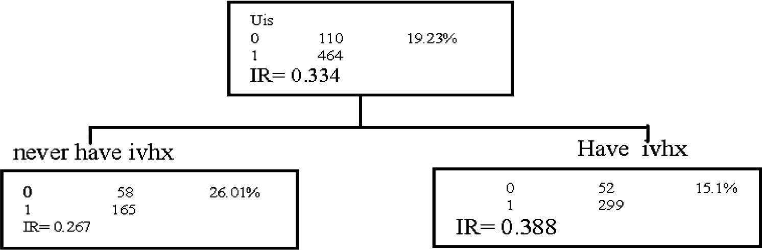

Close

Figure 1

The incidence rate value.

Export to PPT

6.1.2

6.1.2 Level 2

The same algorithm applies to each of the subgroups by using forward technique again to determine the most important covariate. We find that age is the most important covariate for the left node. As it is done in level 1, according to age category, we split the ivhx1 data into two parts then we will get two files “age 2 for young” and “age 1 for old” (we get two nodes).

For the right node, we find the most important covariate is race, and then we split the ivhx2 data into two parts according to race category.

6.1.3

6.1.3 Level 3

Repeating the same procedure till we get either a small group size, or no additional splitting is available (there is not any important covariate). The decision tree that is complete has seven terminals, is shown in Fig. 2.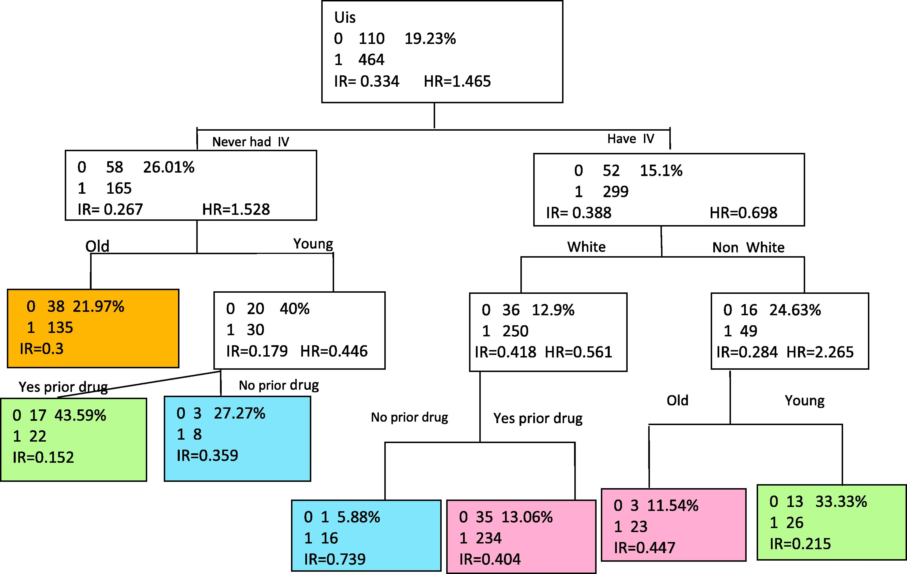

Close

Figure 2

The complete decision tree showing seven terminals.

Export to PPT

6.2

6.2 Plotting the survival curves for terminals

Assign a number for each terminal depending on its incidence rate value, in descending form. This gives the graph of the survival distribution function for the node terminals which is given in Fig. 3.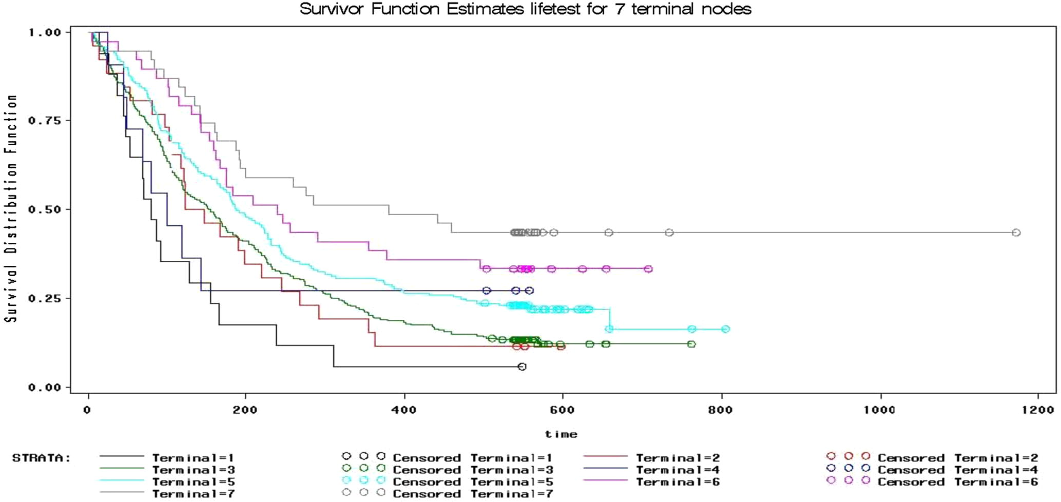

Close

Figure 3

Survival function estimates for the seven terminal nodes.

Export to PPT

7 The conclusion: interpreting the results

The average number of old patients (age >34) who never had IV and return to drug use is 0.3 patients/day.

The average number of young patients (age <34) who never had IV and never had any prior drug treatments and return to drug use is, 0.359 patients/day while, if they had prior drug treatments the average number decreases to 0.152 patients/day.

The average number of young non-white patients who had recent IV and return to drug use is 0.447 patients/day but for the older patients it is only 0.215 patients/day.

The average number of white patients who had recent IV but never had a previous drug treatments and return to drug use is, 0.739 patients/day where as the patient who had prior drug treatments give an average of 0.404 patients/day.

Moreover, we could study the social behavior of these groups (knowing the postal code) to determine the factors which made them in the same group. However, we need the complete data (all covariates related to the events such as marital status, economic level and some medical information) for more analysis.

References

- Classification and Regression Trees. Belmont, CA: Wadsworth; 1984.
- Tree-structured prediction for censored survival data and the cox model. Journal of Clinical Epidemiology. 1995;48(5):675-689.
- [Google Scholar]
- Regression models and life-tables (with discussion) Journal of the Royal Statistical Society, Series, B. 1972;34:187-220.
- Applied Survival Analysis: Regression Modeling of Time to Event Data (second ed.). John Wiley and Sons Inc.; 2008.
- Statistical Models and Methods for Lifetime Data. John Wiley and Sons Inc.; 2003.
- Survival trees by goodness of splits. Journal of the American Statistical Association. 1993;88:457-467.
- Statistical Methods for Survival Data Analysis (third ed.). NY: John Wiley; 2003.
- Problems in analysis of survey data and a proposal. Journal of the American Statistical Association. 1963;58:415-434.
- The Statistical Analysis of Failure Time Data (second ed.). NY: John Wiley; 2002.
- SAS Institute Inc., 2002–2003. Cary, NC, USA, Version 9.1.