Kumaraswamy generalized Kappa distribution with application to stream flow data

Tahir Nawaz; Sajid Hussain; Tanvir Ahmad; Farah Naz; Muhammad Abid

doi:10.1016/j.jksus.2018.04.005

View/Download PDF

Buy Reprints

PDF

Translate this page into:

Original article

32 (

); 172-182

doi:

10.1016/j.jksus.2018.04.005

Kumaraswamy generalized Kappa distribution with application to stream flow data

Tahir Nawaz^⁎, Sajid Hussain, Tanvir Ahmad, Farah Naz, Muhammad Abid

Department of Statistics, Government College University, Faisalabad, Pakistan

⁎Corresponding author. tahir.nawaz@gcuf.edu.pk (Tahir Nawaz),

Received: 2018-3-2, Accepted: 2018-4-4, Published: 2018-01-01

Disclaimer:
This article was originally published by Elsevier and was migrated to Scientific Scholar after the change of Publisher.

Peer review under responsibility of King Saud University.

Abstract

Recently in literature many families of distributions have been introduced to study the skewness, kurtosis and to explore the shape of the distribution more intensely. These families of distribution have wider applicability in variety of fields. In this paper, we introduce a five-parameter distribution, called the Kumaraswamy generalized Kappa distribution which extends the three-parameter Kappa distribution. The new distribution is more flexible and is applicable in the study of the highly-skewed data. Some mathematical properties of the proposed distribution are studied that includes the explicit expression for generating functions, moments, inequality indices, and entropies. The maximum likelihood estimates are computed using the numerical procedure. An application of the Kumaraswamy generalized Kappa distribution is illustrated using a real data set on stream flow.

Keywords

Entropy

Inequality indices

Kumaraswamy distribution

Kappa distribution

Maximum likelihood

Show Related Articles from PubMed

1 Introduction

Many families of distribution have been recently proposed which are more flexible and have wider applicability ranging from survival analysis, reliability engineering, and related fields. Classical distributions do not provide adequate fits to the real data which are highly skewed. To overcome this drawback numerous methods of introducing additional shape parameters, and generating new families of distributions are available in the statistical literature.

Some well-known generators are the Marshall and Olkin (1997), exponentiated generalized (exp-G) class of distributions based on Lehmann-type alternatives suggested by Gupta et al. (1998), generalized-exponential (GE) also known as exponentiated exponential (EE) distributions introduced by Gupta and Kundu (1999), beta-generated distributions proposed by Eugene et al. (2002) and Jones (2004), Kumaraswamy generalized (Kum-G) distribution suggested by Cordeiro and de Castro (2011), McDonald generalized (Mc-G) distribution introduced by Alexander et al. (2012), gamma-generated type-1 distributions proposed by Zografos and Balakrishnan (2009) and Amini et al. (2014), gamma-generated type-2 distributions by Ristic and Balakrishnan (2012) and Amini et al. (2014), exponentiated generalized (exp-G) distribution introduced by Cordeiro et al. (2013) and odd Weibull-generated distribution proposed by Bourguignon et al. (2014). The induction of one, two or three more shape parameters to the base-line distribution increases the chances to investigate skewness and vary tail weights. The earlier mentioned generalizations also help to deduce sub-model of generalized distributions that greatly enhances the applicability.

There is no general class of distribution to model skewed data in every practical situation. Mielke (1973) presented a class of asymmetric positively skewed distributions, known as the Kappa distribution, for explaining and examining rainfall data and weather modification. Mielke and Johnson (1973) presented the maximum likelihood estimates and the likelihood ratio tests for the three-parameter Kappa distribution. The Kappa distribution has obtained attention from the hydrologic experts. Conventionally, the log normal and gamma distributions are fitted to precipitation data but these distributions have their own limitations due to non-existence of closed forms of the cdfs and quantile functions. The class of Kappa distribution have closed algebraic expressions that can easily be analysed.

Let $X$ be a three-parameter Kappa random variable, then the pdf and cdf of the Kappa distribution are given by

(1.1)

f (x) = \frac{α θ}{β} {(\frac{x}{β})}^{θ - 1} {[α + {(\frac{x}{β})}^{α θ}]}^{- \frac{(α + 1)}{α}}

and

(1.2)

F (x) = {[\frac{{(\frac{x}{β})}^{α θ}}{α + {(\frac{x}{β})}^{α θ}}]}^{\frac{1}{α}}

α, β, θ > 0

and

x > 0

Parameter $β$ is scale while parameters $α$ and $θ$ are shape.

In this paper [deduced from Hussain (2015)], we have extended the three parameter Kappa distribution, namely the Kumaraswamy generalized Kappa (KGK) distribution by introducing additional shape parameters. The paper is organized as follows. In Section 2 we have defined KGK distribution, its sub-models and the behaviour of its pdf. The mathematical properties such as: quantile functions, moments, and generating functions are derived in Section 3. The Reliability properties are presented in Section 4. Some inequality indices are given in Section 5. Entropies are discussed in Section 6. Maximum likelihood estimation of the parameters of the distribution is presented in Section 7. The application on real life data set of stream flows amount is provided in Section 8. Finally, Section 9 concludes the manuscript.

2 Kumaraswamy generalized Kappa distribution

Cordeiro and de Castro (2011) defined a general class of general distributions for double-bounded random process based on Kumaraswamy (1980) which is known as the Kumaraswamy generalized (Kum-G) distribution.Let X be a random variable, the cdf of Kum-G class of distribution is given by

(2.1)

F_{Kum - G} (x) = 1 - {[1 - {F (x)}^{a}]}^{b}

where

a

and

b

are additional shape parameters to generalized distribution, which govern skewness and tail weights. The probability density function

(pdf)

corresponding to (2.1) is

(2.2)

f_{Kum - G} (x) = abf (x) {F (x)}^{a - 1} {[1 - {F (x)}^{a}]}^{b - 1}

Inserting (1.2) in (2.1), the

cdf

of the Kumaraswamy generalized Kappa (KGK) distribution is given by

(2.3)

F_{KGK} (x) = 1 - {[1 - {\{\frac{{(\frac{x}{β})}^{α θ}}{α + {(\frac{x}{β})}^{α θ}}\}}^{\frac{a}{α}}]}^{b}; x > 0

The

pdf

corresponding to (2.3), will be

(2.4)

f_{KGK} (x) = ab \frac{α θ}{β} {(\frac{x}{β})}^{θ - 1} {\{α + {(\frac{x}{β})}^{α θ}\}}^{- \frac{(α + 1)}{α}} {\{\frac{{(\frac{x}{β})}^{α θ}}{α + {(\frac{x}{β})}^{α θ}}\}}^{\frac{a - 1}{α}} {[1 - {\{\frac{{(\frac{x}{β})}^{α θ}}{α + {(\frac{x}{β})}^{α θ}}\}}^{\frac{a}{α}}]}^{b - 1}; x > 0

with

a, b, α, β, θ > 0

, where

a, b, α

and

θ

are shape parameters while

β

is scale parameter.

2.1

2.1 Special sub-models

The KGK has the following distributions as special sub-models.

Exponentiated Kappa Lehmann type II (EK-L2) distribution: If $a = 1$ , the KGK reduces to the exponentiated Kappa (Lehmann type II) distribution with parameters $b, α, β$ and $θ$ .
Exponentiated Kappa Lehmann type I (EK-L1) distribution: If $b = 1$ , the KGK reduces to the exponentiated Kappa (Lehmann type I) distribution with parameters $a, α, β$ and $θ$ .
Three-parameter Kappa distribution: If $a = b = 1$ , the KGK reduces to three-parameter Kappa distribution with parameter $α, β$ and $θ$ .
Two-parameter Kappa distribution: If $a = b = θ = 1$ , the KGK reduces to two-parameter Kappa distribution with parameter $α$ and $β$ .
One-parameter Kappa distribution: If $a = b = θ = β = 1$ , the KGK reduces to one-parameter Kappa distribution with parameter $α$ .

2.2

2.2 A useful representation of KGK density function

Using the binomial expansion, ${(1 - ω)}^{b - 1} = \sum_{j = 0}^{\infty} {(- 1)}^{j} (\begin{matrix} b - 1 \\ j \end{matrix}) ω^{j}$ , where $b$ is real non-integer and $| ω | < 1$ .

The KGK density given in (2.4) in more simplified form can be expressed as

(2.5)

f_{KGK} (x) = ab \sum_{j = 0}^{\infty} {(- 1)}^{j} (\begin{matrix} b - 1 \\ j \end{matrix}) \frac{α θ}{β} {(\frac{x}{β})}^{θ a (j + 1) - 1} {\{α + {(\frac{x}{β})}^{α θ}\}}^{- \frac{a}{α} (j + 1) - 1}

a

is an integer, Eq. (2.5) reveals that KGK density function is equals to Kappa density function multiplied by an infinite power series of

W_{j}

(2.6)

f_{KGK} (x) = W_{j} \frac{α θ}{β} {(\frac{x}{β})}^{θ a (j + 1) - 1} {\{α + {(\frac{x}{β})}^{α θ}\}}^{- \frac{a}{α} (j + 1) - 1}

where

W_{j} = ab \sum_{j = 0}^{\infty} {(- 1)}^{j} (\begin{matrix} b - 1 \\ j \end{matrix})

Graphical representation of the density function for various values of the parameters selected arbitrarily provided in Fig. 1. It can be observed from the Fig. 1 that increasing the value of the shape parameters $(a, b, α, θ)$ the peakedness of the density function tends to increase. Similarly, the increase in the value of the scale parameter $β$ shifts the density function away from the origin.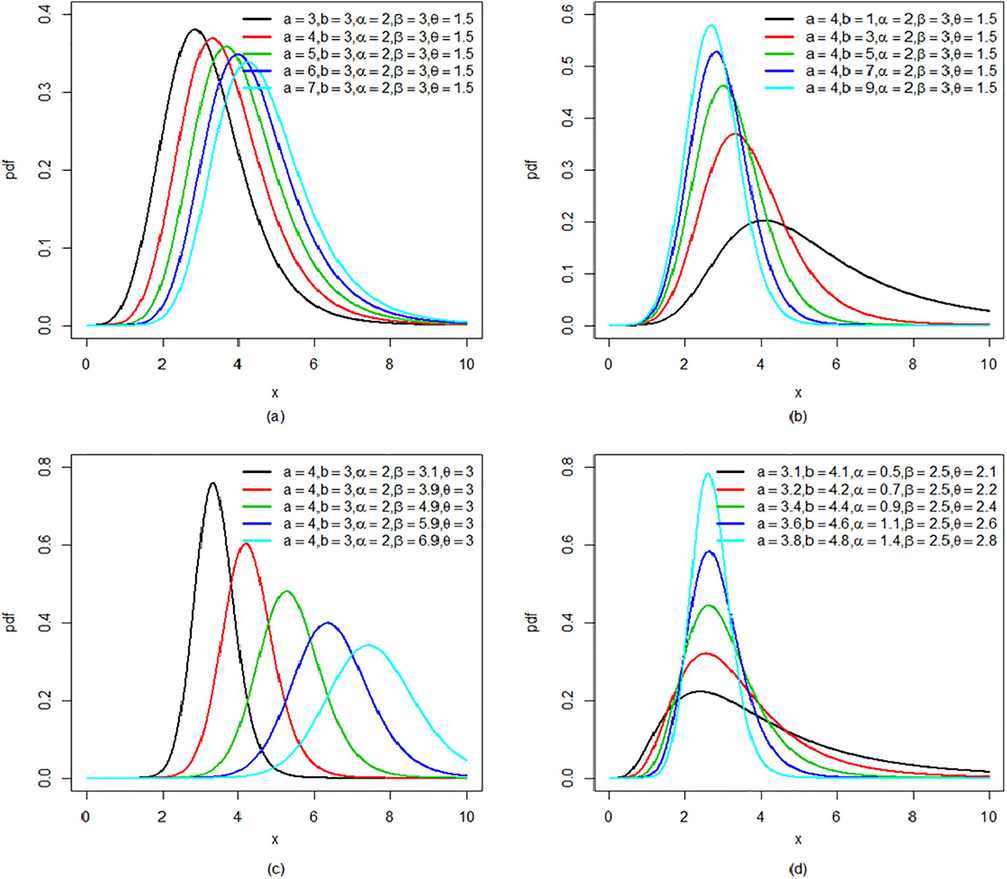

Plots of density function of KGK distribution by varying the parameter values.

3 Statistical properties

In this section, various statistical properties of the KGK distribution, viz. Quantile function, median, random number generation, mode, moments, moment generating function (mgf), characteristic function (cf), mean deviation from mean and mean deviation from median.

3.1

3.1 Quantile function and random number generation

The qth quantile, $x_{q}$ , of the KGK distribution can be obtained by $1 - {[1 - {\{\frac{{(\frac{x_{q}}{β})}^{α θ}}{α + {(\frac{x_{q}}{β})}^{α θ}}\}}^{\frac{a}{α}}]}^{b} = p,$ Now, for solving $x_{q}$ , gives us quantile function of the Kum generalized Kappa (KGK) distribution.

(3.1)

x_{q} = β α^{\frac{1}{α θ}} {\{1 - {(1 - p)}^{\frac{1}{b}}\}}^{\frac{1}{a θ}} {[1 - {\{1 - {(1 - p)}^{\frac{1}{b}}\}}^{\frac{α}{a}}]}^{- \frac{1}{α θ}}, 0 < p < 1

The median

(Q_{2})

of the KGK distribution will be

(3.2)

Q_{2} = x_{0.50} = β α^{\frac{1}{α θ}} {\{1 - {(1 - 0.50)}^{\frac{1}{b}}\}}^{\frac{1}{a θ}} {[1 - {\{1 - {(1 - 0.50)}^{\frac{1}{b}}\}}^{\frac{α}{a}}]}^{- \frac{1}{α θ}}

The lower quartile

(Q_{1})

and upper quartile

(Q_{3})

of the KGK distribution are

Q_{1} = x_{0.25} = β α^{\frac{1}{α θ}} {\{1 - {(1 - 0.25)}^{\frac{1}{b}}\}}^{\frac{1}{a θ}} {[1 - {\{1 - {(1 - 0.25)}^{\frac{1}{b}}\}}^{\frac{α}{a}}]}^{- \frac{1}{α θ}}

and

Q_{3} = x_{0.75} = β α^{\frac{1}{α θ}} {\{1 - {(1 - 0.75)}^{\frac{1}{b}}\}}^{\frac{1}{a θ}} {[1 - {\{1 - {(1 - 0.75)}^{\frac{1}{b}}\}}^{\frac{α}{a}}]}^{- \frac{1}{α θ}}

By the inversion method, the random numbers from KGK distribution can be generated as

1 - {[1 - {\{\frac{{(\frac{x}{β})}^{α θ}}{α + {(\frac{x}{β})}^{α θ}}\}}^{\frac{a}{α}}]}^{b} = u; u \sim U (0, 1)

After simplification, we get

(3.3)

x_{u} = β α^{\frac{1}{α θ}} {\{1 - {(1 - u)}^{\frac{1}{b}}\}}^{\frac{1}{a θ}} {[1 - {\{1 - {(1 - u)}^{\frac{1}{b}}\}}^{\frac{α}{a}}]}^{- \frac{1}{α θ}}

3.2

3.2 Mode

The mode of the KGK is obtained as $logf (x) = \log (\frac{ab α θ}{β}) + (θ a - 1) \log (\frac{x}{β}) - (\frac{α + a}{α}) \log \{α + {(\frac{x}{β})}^{α θ}\} + (b - 1) \times \log [1 - {\{\frac{{(\frac{x}{β})}^{α θ}}{α + {(\frac{x}{β})}^{α θ}}\}}^{\frac{a}{α}}]$ The first derivative of $logf (x)$ for the KGK distribution is $\frac{\partial}{\partial x} logf (x)$ . So, the modes of the KGK distribution are the roots of the following equation $\frac{\partial}{\partial x} logf (x) = 0$ which gives

(3.4)

\frac{θ a - 1}{x} - \frac{θ (α + a) {(\frac{x}{β})}^{α θ - 1}}{β [α + {(\frac{x}{β})}^{α θ}]} - \frac{a (b - 1) α θ {(\frac{x}{β})}^{a θ - 1}}{β [{\{α + {(\frac{x}{β})}^{α θ}\}}^{\frac{a}{α} + 1} - α {(\frac{x}{β})}^{a θ} - {(\frac{x}{β})}^{θ (α + a)}]} = 0

There may be more than one root to Eq. (3.4). If

x = x_{0}

is a root of Eq. (3.4) then it corresponds to a local maximum or local minimum or a point of inflection depending on whether

\frac{\partial^{2}}{\partial x^{2}} logf (x) < or > or = 0

, respectively.

3.3

3.3 rth moment

The $r th$ moment for KGK random variable $X$ is given by $μ_{r}^{'} = E (X^{r}) = \int_{- \infty}^{\infty} x^{r} f_{KGK} (x) dx$ using (2.6), we have $μ_{r}^{'} = \int_{0}^{\infty} x^{r} W_{j} \frac{α θ}{β} {(\frac{x}{β})}^{θ a (j + 1) - 1} {\{α + {(\frac{x}{β})}^{α θ}\}}^{- \frac{a}{α} (j + 1) - 1} dx$ Let $Z = {(\frac{x}{β})}^{α θ}$ then $dx = \frac{β Z^{\frac{1}{α θ}}}{α θ Z} dZ$ After simplification, we get $μ_{r}^{'} = W_{j} \frac{β^{r}}{α^{\frac{a}{α} (j + 1) + 1}} \int_{0}^{\infty} Z^{\frac{r}{α θ} + \frac{a}{α} (j + 1) - 1} {[1 - \{1 - {(1 + \frac{Z}{α})}^{- 1}\}]}^{\frac{a}{α} (j + 1) + 1} dZ$ Let $W = 1 - {(1 + \frac{Z}{α})}^{- 1}$ and $dZ = \frac{α}{{(1 - W)}^{2}} dW$

After simplification, we get $μ_{r}^{'} = W_{j} β^{r} α^{\frac{r}{α θ} - 1} \int_{0}^{1} W^{\frac{r}{α θ} + \frac{a}{α} (j + 1) - 1} {[1 - W]}^{1 - \frac{r}{α θ} - 1} dW$ Using beta function,

(3.5)

μ_{r}^{'} = W_{j} β^{r} α^{\frac{r}{α θ} - 1} B (\frac{r}{α θ} + \frac{a}{α} (j + 1), 1 - \frac{r}{α θ}); r = 1, 2, 3, 4

where

B (a, b) = \int_{0}^{1} U^{a - 1} {[1 - U]}^{b - 1} dU

is the beta function.

The mean and the variance of the KGK distribution are, respectively, given by

(3.6)

mean = W_{j} β α^{\frac{1}{α θ} - 1} B (\frac{1}{α θ} + \frac{a}{α} (j + 1), 1 - \frac{1}{α θ})

(3.7)

Variance = W_{j} β^{2} α^{\frac{2}{α θ} - 1} B (\frac{2}{α θ} + \frac{a}{α} (j + 1), 1 - \frac{2}{α θ}) - {[W_{j} β α^{\frac{1}{α θ} - 1} B (\frac{1}{α θ} + \frac{a}{α} (j + 1), 1 - \frac{1}{α θ})]}^{2}

where

W_{j} = ab \sum_{j = 0}^{\infty} {(- 1)}^{j} (\begin{matrix} b - 1 \\ j \end{matrix})

3.4

3.4 Moment generating function and characteristic function

The moment generating function and characteristic function of the KGK distribution are given by

(3.8)

M (t) = E (e^{tx}) = \sum_{r = 0}^{\infty} \frac{t^{r}}{r!} μ_{r}^{'} = \sum_{r = 0}^{\infty} \frac{t^{r}}{r!} W_{j} β^{r} α^{\frac{r}{α θ} - 1} B (\frac{r}{α θ} + \frac{a}{α} (j + 1), 1 - \frac{r}{α θ}); r = 1, 2, 3, 4

and

(3.9)

φ (t) = E (e^{itx}) = \sum_{r = 0}^{\infty} \frac{{(it)}^{r}}{r!} μ_{r}^{'} = \sum_{r = 0}^{\infty} \frac{{(it)}^{r}}{r!} W_{j} β^{r} α^{\frac{r}{α θ} - 1} B (\frac{r}{α θ} + \frac{a}{α} (j + 1), 1 - \frac{r}{α θ}); r = 1, 2, 3, 4

where

W_{j} = ab \sum_{j = 0}^{\infty} {(- 1)}^{j} (\begin{matrix} b - 1 \\ j \end{matrix})

4 Reliability properties

In this section, we have derived the reliability properties such as survival (or reliability) function, hazard rate, reversed hazard rate, cumulative hazard rate, mean residual life and mean waiting time for the Kumaraswamy generalized Kappa distribution.

A life time random variable $t$ is said to have KGK $(a, b, α, β, θ)$ distribution, when its $cdf$ and $pdf$ are represented as follows

(4.1)

F_{KGK} (t) = 1 - {[1 - {\{\frac{{(\frac{t}{β})}^{α θ}}{α + {(\frac{t}{β})}^{α θ}}\}}^{\frac{a}{α}}]}^{b}; t > 0

and

(4.2)

f_{KGK} (t) = ab \frac{α θ}{β} {(\frac{t}{β})}^{θ a - 1} {\{α + {(\frac{t}{β})}^{α θ}\}}^{- \frac{(α + a)}{α}} {[1 - {\{\frac{{(\frac{t}{β})}^{α θ}}{α + {(\frac{t}{β})}^{α θ}}\}}^{\frac{a}{α}}]}^{b - 1}

t > 0

a, b, α, β, θ > 0

The survival (or reliability) function, $S (t)$ , is given by

(4.3)

S (t) = 1 - F (t) = {[1 - {\{\frac{{(\frac{t}{β})}^{α θ}}{α + {(\frac{t}{β})}^{α θ}}\}}^{\frac{a}{α}}]}^{b}

The failure rate or hazard rate function,

h (t)

, for KGK distribution is given by

(4.4)

h (t) = \frac{f (t)}{S (t)} = ab \frac{α θ}{β} {(\frac{t}{β})}^{θ a - 1} {\{α + {(\frac{t}{β})}^{α θ}\}}^{- \frac{(α + a)}{α}} {[1 - {\{\frac{{(\frac{t}{β})}^{α θ}}{α + {(\frac{t}{β})}^{α θ}}\}}^{\frac{a}{α}}]}^{- 1}

Various shape of the hazard function for different parameter values are presented in Fig. 2.

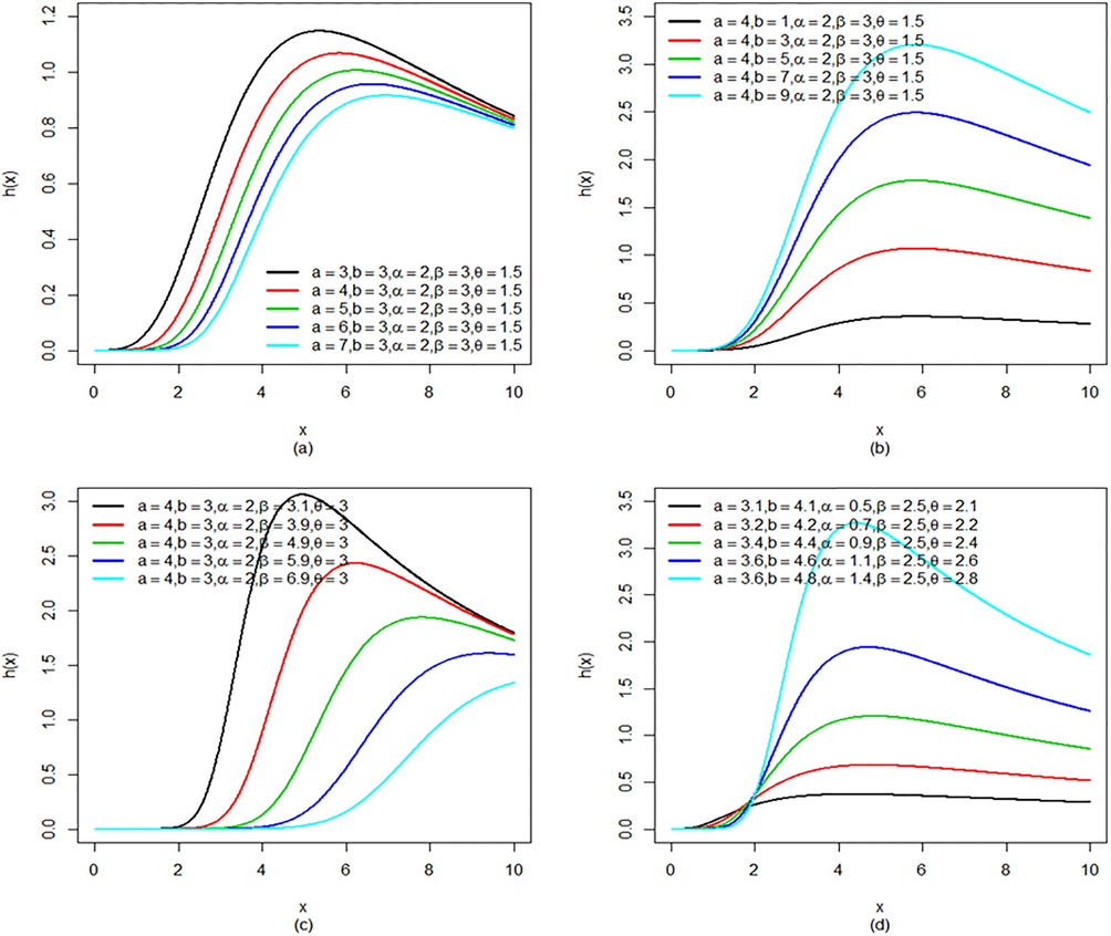
Plots of hazard rate of KGK distribution by varying the parameter values.

It is observable from Fig. 2 that the hazard rate of the KGK distribution tends to increase initially, and then after reaching a certain level it starts decreasing. This indicates that the KGK distribution can be useful to model first increasing then decreasing hazard rate.

The cumulative hazard rate function, $H (t)$ , and reversed hazard rate, $r (t)$ , of KGK distribution are given respectively as

(4.5)

H (t) = \int_{0}^{t} h (t) dt = - lnS (t) = - bln [1 - {\{\frac{{(\frac{t}{β})}^{α θ}}{α + {(\frac{t}{β})}^{α θ}}\}}^{\frac{a}{α}}]

and

(4.6)

r (t) = \frac{f (t)}{F (t)} = \frac{ab \frac{α θ}{β} {(\frac{t}{β})}^{θ a - 1} {\{α + {(\frac{t}{β})}^{α θ}\}}^{- \frac{(α + a)}{α}} {[1 - {\frac{{(\frac{t}{β})}^{α θ}}{α + {(\frac{t}{β})}^{α θ}}}^{\frac{a}{α}}]}^{b - 1}}{1 - {[1 - {\{\frac{{(\frac{t}{β})}^{α θ}}{α + {(\frac{t}{β})}^{α θ}}\}}^{\frac{a}{α}}]}^{b}}

The mean residual life (MRL) or life expectancy at a given time

t

measures the expected remaining life time of an individual of age

t

. It is defined as

(4.7)

m (t) = \frac{1}{S (t)} \int_{t}^{\infty} tf (t) dt - t

which can also be written as

m (t) = \frac{1}{S (t)} \{E (t) - \int_{0}^{t} tf (t) dt\} - t

Now consider

\int_{t}^{\infty} tf (t) dt = \int_{t}^{\infty} {tW}_{j} \frac{α θ}{β} {(\frac{t}{β})}^{θ a (j + 1) - 1} {\{α + {(\frac{t}{β})}^{α θ}\}}^{- \frac{a}{α} (j + 1) - 1} dt

After simplification and using incomplete beta function, we get

(4.8)

= W_{j} β α^{\frac{1}{α θ} - 1} B (\frac{a}{α} (j + 1) + \frac{1}{α θ}, 1 - \frac{1}{α θ}) - W_{j} β α^{\frac{1}{α θ} - 1} B_{W} (\frac{a}{α} (j + 1) + \frac{1}{α θ}, 1 - \frac{1}{α θ})

where

W = 1 - {(1 + \frac{Z}{α})}^{- 1}

Z = {(\frac{t}{β})}^{α θ}

and

B_{W} (a, b) = \int_{0}^{t} t^{a - 1} {[1 - t]}^{b - 1} dt

is the incomplete beta function.

Using the results of (4.8) in (4.7), the MRL of the KGK distribution obtained as

(4.9)

m (t) = \frac{W_{j} β α^{\frac{1}{α θ} - 1} [B (\frac{a}{α} (j + 1) + \frac{1}{α θ}, 1 - \frac{1}{α θ}) - B_{W} (\frac{a}{α} (j + 1) + \frac{1}{α θ}, 1 - \frac{1}{α θ})]}{{[1 - {\{\frac{{(\frac{t}{β})}^{α θ}}{α + {(\frac{t}{β})}^{α θ}}\}}^{\frac{a}{α}}]}^{b}} - t

The mean waiting time (MWT) of an item failed in an interval

[0, t]

is defined as

(4.10)

\bar{μ} (t, θ^{'}) = t - \{\frac{1}{F (t)} \int_{0}^{t} tf (t) dt\}

The MWT of the KGK distribution is given as

(4.11)

\bar{μ} (t, θ^{'}) = t - [W_{j} β α^{\frac{1}{α θ} - 1} B_{W} (\frac{a}{α} (j + 1) + \frac{1}{α θ}, 1 - \frac{1}{α θ})] {[1 - {[1 - {\{\frac{{(\frac{t}{β})}^{α θ}}{α + {(\frac{t}{β})}^{α θ}}\}}^{\frac{a}{α}}]}^{b}]}^{- 1}

5 Inequality measures

In this section, inequality measures such as Gini index, Lorenz curve, Bonferroni curve, Zenga index, Atkinson index, Pietra index and generalized entropy for the KGK distribution have been obtained.

5.1

5.1 Gini index

The most well-known inequality index is Gini index, suggested by Gini (1914), is defined as

(5.1)

G = \frac{1}{E (x)} \int_{0}^{\infty} F (x) {1 - F (x)} dx

Consider

(5.2)

F (x) {1 - F (x)} = {[1 - {\{\frac{{(\frac{x}{β})}^{α θ}}{α + {(\frac{x}{β})}^{α θ}}\}}^{\frac{a}{α}}]}^{b} - {[1 - {\{\frac{{(\frac{x}{β})}^{α θ}}{α + {(\frac{x}{β})}^{α θ}}\}}^{\frac{a}{α}}]}^{2 b}

Now integrating and applying binomial expansion on (5.2) for KGK distribution, we get

\int_{0}^{\infty} F (x) {1 - F (x)} dx = \int_{0}^{\infty} W_{i} {\{\frac{{(\frac{x}{β})}^{α θ}}{α + {(\frac{x}{β})}^{α θ}}\}}^{\frac{a}{α} i} dx - \int_{0}^{\infty} W_{k} {\{\frac{{(\frac{x}{β})}^{α θ}}{α + {(\frac{x}{β})}^{α θ}}\}}^{\frac{a}{α} k} dx

where

W_{i} = \sum_{i = 0}^{\infty} {(- 1)}^{i} (\begin{matrix} b \\ i \end{matrix})

and

W_{k} = \sum_{k = 0}^{\infty} {(- 1)}^{k} (\begin{matrix} 2 b \\ k \end{matrix})

Now simplifying further, we have

(5.3)

\int_{0}^{\infty} F (x) {1 - F (x)} dx = W_{i} \int_{0}^{\infty} {\{\frac{{(\frac{x}{β})}^{α θ}}{α + {(\frac{x}{β})}^{α θ}}\}}^{\frac{a}{α} i} dx - W_{k} \int_{0}^{\infty} {\{\frac{{(\frac{x}{β})}^{α θ}}{α + {(\frac{x}{β})}^{α θ}}\}}^{\frac{a}{α} k} dx

Using transformation,

Z = {(\frac{x}{β})}^{α θ}

such that

dx = \frac{β}{α θ} Z^{\frac{1}{α θ} - 1} dZ

we may write,

(5.4)

= \frac{β}{α θ} [\frac{W_{i}}{α^{\frac{a}{α} i}} \int_{0}^{\infty} Z^{\frac{a}{α} i + \frac{1}{α θ} - 1} {[1 - \{1 - {(1 + \frac{Z}{α})}^{- 1}\}]}^{\frac{a}{α} i} dZ - \frac{W_{k}}{α^{\frac{a}{α} k}} \int_{0}^{\infty} Z^{\frac{a}{α} k + \frac{1}{α θ} - 1} {[1 - \{1 - {(1 + \frac{Z}{α})}^{- 1}\}]}^{\frac{a}{α} k} dZ]

Let

W = 1 - {(1 + \frac{Z}{α})}^{- 1}

then

dZ = \frac{α}{{(1 - W)}^{2}} dW

.Then (5.4) becomes

(5.5)

\int_{0}^{\infty} = \frac{β α^{\frac{1}{α θ} - 1}}{θ} [W_{i} \int_{0}^{1} W^{\frac{a}{α} i + \frac{1}{α θ} - 1} {[1 - W]}^{- \frac{1}{α θ} - 1} dW - W_{k} \int_{0}^{1} W^{\frac{a}{α} k + \frac{1}{α θ} - 1} {[1 - W]}^{- \frac{1}{α θ} - 1} dW]

Using beta function, we get

(5.6)

\int_{0}^{\infty} F (x) {1 - F (x)} dx = \frac{β α^{\frac{1}{α θ} - 1}}{θ} [W_{i} B (\frac{a}{α} i + \frac{1}{α θ}, - \frac{1}{α θ}) - W_{k} B (\frac{a}{α} k + \frac{1}{α θ}, - \frac{1}{α θ})]

Substituting the results of (5.6) and (3.6) in (5.1), the Gini index for KGK distribution obtained as

(5.7)

G = \frac{[W_{i} B (\frac{a}{α} i + \frac{1}{α θ}, - \frac{1}{α θ}) - W_{k} B (\frac{a}{α} k + \frac{1}{α θ}, - \frac{1}{α θ})]}{θ W_{j} B (\frac{1}{α θ} + \frac{a}{α} (j + 1), 1 - \frac{1}{α θ})}

where

W_{i} = \sum_{i = 0}^{\infty} {(- 1)}^{i} (\begin{matrix} b \\ i \end{matrix})

W_{k} = \sum_{k = 0}^{\infty} {(- 1)}^{k} (\begin{matrix} 2 b \\ k \end{matrix})

W_{j} = ab \sum_{j = 0}^{\infty} {(- 1)}^{j} (\begin{matrix} b - 1 \\ j \end{matrix})

and

E (x) = W_{j} β α^{\frac{1}{α θ} - 1} B (\frac{1}{α θ} + \frac{a}{α} (j + 1), 1 - \frac{1}{α θ})

is the mean of KGK distribution.

5.2

5.2 Lorenz curve

Lorenz (1905) provided a curve, $L (p)$ , which is defined as

(5.8)

L (p) = \frac{1}{μ} \int_{0}^{x} xf (x) dx

having a cdf,

F (x)

, with a finite mean

μ

The $L (p)$ for KGK distribution is given as

(5.9)

L (p) = \frac{B_{W} (\frac{a}{α} (j + 1) + \frac{1}{α θ}, 1 - \frac{1}{α θ})}{B (\frac{a}{α} (j + 1) + \frac{1}{α θ}, 1 - \frac{1}{α θ})}

5.3

5.3 Bonferroni curve

The curve suggested by Bonferroni (1930) based on partial means for inequality measure can be determined through the relation

(5.10)

BC (p) = \frac{L (p)}{F (x)}

Using (5.9) and (2.3), we obtain

BC (p)

for KGK distribution as

(5.11)

BC (p) = {[1 - {[1 - {\{\frac{{(\frac{x}{β})}^{α θ}}{α + {(\frac{x}{β})}^{α θ}}\}}^{\frac{a}{α}}]}^{b}]}^{- 1} [\frac{B_{W} (\frac{a}{α} (j + 1) + \frac{1}{α θ}, 1 - \frac{1}{α θ})}{B (\frac{a}{α} (j + 1) + \frac{1}{α θ}, 1 - \frac{1}{α θ})}]

5.4

5.4 Zenga index

Zenga (1984, 1990) provided the following income inequality index

(5.12)

Z = 1 - \frac{μ_{(x)}^{-}}{μ_{(x)}^{+}}

where

(5.13)

μ_{(x)}^{-} = \frac{1}{F (x)} \int_{0}^{x} xf (x) dx

and

(5.14)

μ_{(x)}^{+} = \frac{1}{1 - F (x)} \int_{x}^{\infty} xf (x) dx

which can also be written as

(5.15)

μ_{(x)}^{+} = \frac{1}{1 - F (x)} \{μ - \int_{0}^{x} xf (x) dx\}

For KGK distribution, we obtain

(5.16)

μ_{(x)}^{-} = [W_{j} β α^{\frac{1}{α θ} - 1} B_{W} (\frac{a}{α} (j + 1) + \frac{1}{α θ}, 1 - \frac{1}{α θ})] {[1 - {[1 - {\{\frac{{(\frac{x}{β})}^{α θ}}{α + {(\frac{x}{β})}^{α θ}}\}}^{\frac{a}{α}}]}^{b}]}^{- 1}

and

(5.17)

μ_{(x)}^{+} = [μ - W_{j} β α^{\frac{1}{α θ} - 1} B_{W} (\frac{a}{α} (j + 1) + \frac{1}{α θ}, 1 - \frac{1}{α θ})] {[1 - {\{\frac{{(\frac{x}{β})}^{α θ}}{α + {(\frac{x}{β})}^{α θ}}\}}^{\frac{a}{α}}]}^{- b}

Now, from (5.16) and (5.17), the Zenga index obtained for KGK distribution is

(5.18)

Z = 1 - [\frac{W_{j} β α^{\frac{1}{α θ} - 1} B_{W} (\frac{a}{α} (j + 1) + \frac{1}{α θ}, 1 - \frac{1}{α θ})}{μ - W_{j} β α^{\frac{1}{α θ} - 1} B_{W} (\frac{a}{α} (j + 1) + \frac{1}{α θ}, 1 - \frac{1}{α θ})}] {[{[1 - {\{\frac{{(\frac{x}{β})}^{α θ}}{α + {(\frac{x}{β})}^{α θ}}\}}^{\frac{a}{α}}]}^{- b} - 1]}^{- 1}

5.5

5.5 Atkinson index

Atkinson (1970) presented a family of subjective indices, is defined as

(5.19)

A_{F} (θ^{'}, ε) = 1 - \frac{1}{μ} {\{\int_{0}^{\infty} x^{1 - ε} dF (x)\}}^{\frac{1}{1 - ε}}

which can also be written as

(5.20)

A_{F} (θ^{'}, ε) = 1 - \frac{1}{μ} {μ_{1 - ε}^{'}}^{\frac{1}{1 - ε}}

Using (3.5), we get

(5.21)

μ_{1 - ε}^{'} = W_{j} β^{1 - ε} α^{\frac{1 - ε}{α θ} - 1} B (\frac{1 - ε}{α θ} + \frac{a}{α} (j + 1), 1 - \frac{1 - ε}{α θ})

Using (3.6) and (5.21), the Atkinson index obtained for KGK distribution is

(5.22)

A_{F} (θ^{'}, ε) = 1 - \frac{{\{W_{j} β^{1 - ε} α^{\frac{1 - ε}{α θ} - 1} B (\frac{1 - ε}{α θ} + \frac{a}{α} (j + 1), 1 - \frac{1 -}{α θ})\}}^{\frac{1}{1 - ε}}}{W_{j} β α^{\frac{1}{α θ} - 1} B (\frac{1}{α θ} + \frac{a}{α} (j + 1), 1 - \frac{1}{α θ})}

5.6

5.6 Pietra index

Pietra (1915) offered an index, which is also known as Schutz index or half the relative mean deviation is defined as

(5.23)

P_{X} = \frac{1}{2 μ} \int_{0}^{\infty} | x - μ | dF (x) = \frac{{MD}_{\bar{x}}}{2 μ}

The Pietra index for KGK distribution is

(5.24)

P_{X} = \frac{[μ F (μ) - W_{j} β α^{\frac{1}{α θ} - 1} B_{W} (\frac{a}{α} (j + 1) + \frac{1}{α θ}, 1 - \frac{1}{α θ})]}{W_{j} β α^{\frac{1}{α θ} - 1} B (\frac{a}{α} (j + 1) + \frac{1}{α θ}, 1 - \frac{1}{α θ})}

5.7

5.7 Generalized entropy (GE)

Cowell (1980) and Shorrocks (1980) introduced the generalized entropy (GE) index and is defined as

(5.25)

{GE}_{F} (θ^{'}, δ) = \frac{1}{δ (δ - 1)} \int_{0}^{\infty} \{{(\frac{x}{μ})}^{δ} - 1\} f (x) dx; δ \neq 0, 1

which can also be written as

(5.26)

{GE}_{F} (θ^{'}, δ) = \frac{1}{δ (δ - 1)} \{\frac{μ_{δ}^{'}}{μ^{δ}} - 1\}

where

μ_{δ}^{'}

is the

δ th

moment about origin.

Using (3.5), we get

(5.27)

μ_{δ}^{'} = W_{j} β^{δ} α^{\frac{δ}{α θ} - 1} B (\frac{a}{α} (j + 1) + \frac{δ}{α θ}, 1 - \frac{δ}{α θ})

Now, inserting the results of (5.27) and (3.6) in (5.26), the GE obtained for KGK distribution is

(5.28)

{GE}_{F} (θ^{'}, δ) = \frac{1}{δ (δ - 1)} \{\frac{W_{j} β^{δ} α^{\frac{δ}{α θ} - 1} B (\frac{a}{α} (j + 1) + \frac{δ}{α θ}, 1 - \frac{δ}{α θ})}{{(W_{j} β α^{\frac{1}{α θ} - 1} B (\frac{a}{α} (j + 1) + \frac{1}{α θ}, 1 - \frac{1}{α θ}))}^{δ}} - 1\}

δ = 2

in (5.28), we obtain another inequality measures (squared coefficient of variation)

(5.29)

E_{2} (x) = \frac{{CV}^{2}}{2} = \frac{1}{2} \{\frac{W_{j} β^{2} α^{\frac{2}{α θ} - 1} B (\frac{a}{α} (j + 1) + \frac{2}{α θ}, 1 - \frac{2}{α θ})}{{(W_{j} β α^{\frac{1}{α θ} - 1} B (\frac{a}{α} (j + 1) + \frac{1}{α θ}, 1 - \frac{1}{α θ}))}^{2}} - 1\}

6 Entropies

The most essential entropies of $X \sim KGK (a, b, α, β, θ)$ are Shannon entropy, Rényi entropy, $β$ -entropy. Here we consider two entropy measures: the Rényi entropy, $β$ -entropy. Entropies and kurtosis measures play the same role in comparing the shape of various densities and measuring heaviness of tails.

6.1

6.1 Rényi entropy

Rényi (1961) provided an extension of the Shannon entropy which is defined as:

(6.1)

I_{R} (γ) = \frac{1}{1 - γ} \log \{\int f^{r} (x) dx\}

where

γ > 0

and

γ \neq 1

Applying binomial expansion on KGK $pdf$ given by (2.4), we get $f^{γ} (x)$ in more simple form

(6.2)

f^{γ} (x) = {(\frac{ab α θ}{β})}^{γ} \sum_{j = 0}^{\infty} {(- 1)}^{j} (\begin{matrix} γ (b - 1) \\ j \end{matrix}) {(\frac{x}{β})}^{a θ (γ + j) - γ} {\{α + {(\frac{x}{β})}^{α θ}\}}^{- (\frac{a}{α} + 1) γ - \frac{aj}{α}}

The integral in (6.1) becomes

(6.3)

{(\frac{ab α θ}{β})}^{γ} \sum_{j = 0}^{\infty} {(- 1)}^{j} (\begin{matrix} γ (b - 1) \\ j \end{matrix}) \int_{0}^{\infty} {(\frac{x}{β})}^{a θ (γ + j) - γ} {\{α + {(\frac{x}{β})}^{α θ}\}}^{- (\frac{a}{α} + 1) γ - \frac{aj}{α}} dx

By using transformation

W = {(\frac{x}{β})}^{α θ}

such that

dx = \frac{β}{α θ} W^{\frac{1}{α θ} - 1} dW

(6.3) reduces to

(6.4)

\int_{0}^{\infty} f^{γ} (x) dx = {(ab)}^{γ} {(\frac{θ}{β})}^{γ - 1} α^{\frac{1}{α θ} - \frac{γ}{α θ} - 1} \sum_{j = 0}^{\infty} {(- 1)}^{j} (\begin{matrix} γ (b - 1) \\ j \end{matrix}) \int_{0}^{1} Z^{\frac{a}{α} (γ + j) - \frac{γ}{α θ} + \frac{1}{α θ} - 1} {[1 - Z]}^{γ + \frac{γ}{α θ} - \frac{1}{α θ} - 1} dz

Using beta function, (6.4) reduces to

(6.5)

\int_{0}^{\infty} f^{γ} (x) dx = {(ab)}^{γ} {(\frac{θ}{β})}^{γ - 1} α^{\frac{1}{α θ} - \frac{γ}{α θ} - 1} \sum_{j = 0}^{\infty} {(- 1)}^{j} (\begin{matrix} γ (b - 1) \\ j \end{matrix}) B (\frac{a}{α} (γ + j) - \frac{γ}{α θ} + \frac{1}{α θ}, γ + \frac{γ}{α θ} - \frac{1}{α θ})

Substituting the result of (6.5), then (6.1) becomes, the Rényi entropy for KGK distribution is given by

(6.6)

I_{R} (γ) = \frac{1}{1 - γ} \log \{{(ab)}^{γ} {(\frac{θ}{β})}^{γ - 1} α^{\frac{1 - γ}{α θ} - 1} \sum_{j = 0}^{\infty} {(- 1)}^{j} (\begin{matrix} γ (b - 1) \\ j \end{matrix}) B (\frac{a}{α} (γ + j) - \frac{γ}{α θ} + \frac{1}{α θ}, γ + \frac{γ}{α θ} - \frac{1}{α θ})\}

6.2

6.2 $β$ -entropy

Havrda and Charvát (1967) presented $β$ -entropy and later Tsallis (1988) applied it to physical problems. Furthermore, one-parameter generalization of the Shannon entropy is $β$ -entropy which can lead to models or statistical results that are different from those acquired by using the Shannon entropy.

For a continuous random variable $X$ having $pdff (x)$ , the $β$ -entropy is defined by

(6.7)

I_{β^{'}} (γ) = \frac{1}{β^{'} - 1} [1 - \int f^{β^{'}} (x) dx]

where

β^{'} > 0

and

β^{'} \neq 1

Using the result of (6.5), we get

(6.8)

\int_{0}^{\infty} f^{β^{'}} (x) dx = {(ab)}^{β^{'}} {(\frac{θ}{β})}^{β^{'} - 1} α^{\frac{1}{α θ} - \frac{β^{'}}{α θ} - 1} \sum_{j = 0}^{\infty} {(- 1)}^{j} (\begin{matrix} β^{'} (b - 1) \\ j \end{matrix}) B (\frac{a}{α} (β^{'} + j) - \frac{β^{'}}{α θ} + \frac{1}{α θ}, β^{'} + \frac{β^{'}}{α θ} - \frac{1}{α θ})

Hence, the expression for

β

-entropy is given as

(6.9)

I_{β^{'}} (γ) = \frac{1}{β^{'} - 1} [1 - {(ab)}^{β^{'}} {(\frac{θ}{β})}^{β^{'} - 1} α^{\frac{1}{α θ} - \frac{β^{'}}{α θ} - 1} \sum_{j = 0}^{\infty} {(- 1)}^{j} (\begin{matrix} β^{'} (b - 1) \\ j \end{matrix}) B (\frac{a}{α} (β^{'} + j) - \frac{β^{'}}{α θ} + \frac{1}{α θ}, β^{'} + \frac{β^{'}}{α θ} - \frac{1}{α θ})]

7 Estimation of parameters of KGK distribution

This section considers the estimation of the model parameters of the KGK distribution by using the method of maximum likelihood.

We assume that $X$ follows the KGK distribution and let $Θ = (a,b, α, β, θ)$ be the parameter vector of interest. The log-likelihood function $ℓ = L (Θ)$ for a random sample $x_{1}, x_{2}, \dots, x_{n}$ is given by

(7.1)

ℓ = nlog (ab α θ β^{- θ a}) + (θ a - 1) \sum_{i = 1}^{n} {logx}_{i} - (1 + \frac{a}{α}) \sum_{i = 1}^{n} \log [α + {(\frac{x_{i}}{β})}^{α θ}] + (b - 1) \sum_{i = 1}^{n} \log [1 - {\{\frac{{(\frac{x_{i}}{β})}^{α θ}}{α + {(\frac{x_{i}}{β})}^{α θ}}\}}^{\frac{a}{α}}]

Let

Z_{i} = {\{\frac{{(\frac{x_{i}}{β})}^{α θ}}{α + {(\frac{x_{i}}{β})}^{α θ}}\}}^{\frac{1}{α}}

. Then, we can write

ℓ

(7.2)

ℓ = nlog (ab α θ β^{- θ a}) + (θ a - 1) \sum_{i = 1}^{n} {logx}_{i} - (1 + \frac{a}{α}) \sum_{i = 1}^{n} \log [α + {(\frac{x_{i}}{β})}^{α θ}] + (b - 1) \sum_{i = 1}^{n} \log [1 - Z_{i}^{a}]

The components of the score vector

U (Θ)

are given by

U_{a} = \frac{n}{a} (1 - a θ \log β) + θ \sum_{i = 1}^{n} {logx}_{i} - \frac{1}{α} \sum_{i = 1}^{n} \log [α + {(\frac{x_{i}}{β})}^{α θ}] + (1 - b) \sum_{i = 1}^{n} \frac{{logZ}_{i}}{Z_{i}^{- a} - 1}

U_{b} = \frac{n}{b} + \sum_{i = 1}^{n} \log [1 - Z_{i}^{a}]

U_{α} = \frac{n}{α} + \frac{a}{α^{2}} \sum_{i = 1}^{n} \log [α + {(\frac{x_{i}}{β})}^{α θ}] - (1 + \frac{a}{α}) \sum_{i = 1}^{n} {[α + {(\frac{x_{i}}{β})}^{α θ}]}^{- 1} - θ (1 + \frac{a}{α}) \times \sum_{i = 1}^{n} Z_{i}^{α} \log (\frac{x_{i}}{β}) + a (1 - b) \sum_{i = 1}^{n} \frac{Z_{i}^{a - 1} Z_{i α}^{'}}{1 - Z_{i}^{a}}

U_{β} = - \frac{na θ}{β} + \frac{(a + α) θ}{β} \sum_{i = 1}^{n} Z_{i}^{α} + a (1 - b) \sum_{i = 1}^{n} \frac{Z_{i}^{a - 1} Z_{i β}^{'}}{1 - Z_{i}^{a}}

U_{θ} = \frac{n}{θ} (1 - a θ \log β) + a \sum_{i = 1}^{n} {logx}_{i} - (a + α) \sum_{i = 1}^{n} Z_{i}^{α} \log (\frac{x_{i}}{β}) + a (1 - b) \sum_{i = 1}^{n} \frac{Z_{i}^{a - 1} Z_{i θ}^{'}}{1 - Z_{i}^{a}}

To find the MLEs of the five parameters

a, b, α, β

and

θ

. Setting

U_{a}, U_{b}, U_{α}, U_{β}

and

U_{θ}

to zero and solving them simultaneously. For interval estimation of the model parameters, we require the

5 \times 5

observed information matrix

J (Θ) = {U_{s, t}}

where

s, t = a, b, α, β, θ

given in Appendix A. To construct approximate confidence intervals for

a, b, α, β

and

θ

the multivariate normal

N_{5} (0, J {(\hat{Θ})}^{- 1})

distribution can be used under standard regularity conditions. Here,

J (\hat{Θ})

is the total observed information matrix evaluated at

\hat{Θ}

. Then,

100 (1 - α^{*}) %

confidence interval for

a, b, α, β

and

θ

are given by

\hat{a} \pm Z_{α^{*} / 2} σ_{\hat{a}}

\hat{b} \pm Z_{α^{*} / 2} σ_{\hat{b}}

\hat{α} \pm Z_{α^{*} / 2} σ_{\hat{α}}

\hat{β} \pm Z_{α^{*} / 2} σ_{\hat{β}}

and

\hat{θ} \pm Z_{α^{*} / 2} σ_{\hat{θ}}

, respectively, where

Z_{α^{*} / 2}

is the quantile

(1 - α^{*} / 2)

of the standard normal distribution, and

σ_{(\cdot)}

’s denote the diagonal elements of

J {(\hat{Θ})}^{- 1}

corresponding to

a, b, α, β

and

θ

To check KGK distribution is strictly superior to the Kappa distribution for a given data set the likelihood ratio (LR) statistic can be used. Then, the test of $H_{0} : a = b = 1$ versus $H_{1} : H_{0} is not true$ is equivalent to compare the KGK and Kappa distributions and the LR statistic becomes $w = 2 {ℓ (\hat{a}, \hat{b}, \hat{α}, \hat{β}, \hat{θ}) - ℓ (1, 1, \hat{α}, \hat{β}, \hat{θ})}$ , where $\hat{a}, \hat{b}, \hat{α}, \hat{β}$ and $\hat{θ}$ are the MLEs under $H_{1}$ and $\hat{α}, \hat{β}$ and $\hat{θ}$ are the estimates under $H_{0}$ .

8 Empirical illustration

In this section, real data set is examined for illustration purpose. The MLEs are calculated and the measures of goodness of fit are used to compare the proposed model Kumaraswamy generalized Kappa distribution with the other competing models. We computed log-likelihood $ℓ (\cdot)$ , AIC (Akaike information criterion), BIC (Bayesian information criterion) and CAIC (consistent Akaike information criterion): $AIC = - 2 ℓ (\cdot) + 2 p, BIC = - 2 ℓ (\cdot) + plogn, and CAIC = - 2 ℓ (\cdot) + \frac{2 pn}{n - p - 1}$ where $ℓ (\cdot)$ signifies the log-likelihood function examined at the maximum likelihood estimates, $p$ is the number of parameters, and $n$ is the sample size. We also used conventional goodness-of-fit tests in order to check which distribution fits better to this data set. We look at the Cramer-von Mises $(W^{*})$ and Anderson-Darling $(A^{*})$ statistics. In general, the smaller the values of these statistics, the better the fit to the data.

The following data set from Mielke and Johnson (1973) consists of Stream flow amounts (1000 acre-feet) for 35 year (1936–70) at the U.S. Geological Survey (USGS) gaging station number 9-3425 for April 1–August 31 of each year:

192.48, 303.91, 301.26, 135.87, 126.52, 474.25, 297.17, 196.47, 327.64, 261.34, 96.26, 160.52, 314.60, 346.30, 154.44, 111.16, 389.92, 157.93, 126.46, 128.58, 155.62, 400.93, 248.57, 91.27, 238.71, 140.76, 228.28, 104.75, 125.29, 366.22, 192.01, 149.74, 224.58, 242.19, 151.25.

Table 1 presents the estimated values of the MLEs of the parameters of the distributions and their standard errors. Estimated values for AIC, BIC, CAIC, $A^{*}$ and $W^{*}$ against all the fitted distributions are provided in Table 2. The histogram of the data set and the estimated pdfs and cdfs for the fitted models are displayed in Fig. 3. It is evident from the lower value of the statistics $A^{*}$ and $W^{*}$ for KGK distribution in comparison to the rest of the fitted distributions that it is the best fit distribution in the given circumstances. These findings are further supplemented by the estimated pdf and cdf plots given in Fig. 3 which clearly depicts that KGK distribution is a better fitted model as compared to others.

Table 1 MLEs and their standard errors (in parentheses) for Stream flow amounts (1000 acre-feet).

Distribution	$a$	$b$	$α$	$β$	$θ$
KGK	37.6739 (563.6182)	4.8300 (9.7572)	0.1678 (1.0243)	17.3661 (219.7929)	7.2191 (44.7869)
EK (Lehmann type-I)	58.6622 (1716.8957)	– –	0.2164 (1.6786)	32.0895 (373.3277)	11.7289 (91.2334)
EK (Lehmann type-II)	– –	8.3742 (36.9606)	0.0629 (0.1273)	515.3789 (1623.1231)	16.8224 (26.8103)
Kappa3	– –	– –	0.0457 (0.2369)	161.5442 (15.9801)	56.7357 (287.0343)
Kappa2	– –	– –	10.7420 (5.9393)	312.1797 (46.5958)	– –

Table 2 The

ℓ (\cdot)

, AIC, BIC, CAIC,

A^{*}

W^{*}

values for Stream flow amounts (1000 acre-feet).

Distribution	$ℓ (\cdot)$	$AIC$	$BIC$	$CAIC$	$A^{*}$	$W^{*}$
KGK	206.4671	422.9343	430.7110	425.0033	0.4555	0.0788
EK (Lehmann type-I)	207.0059	422.0117	428.2331	423.3450	0.4931	0.0794
EK (Lehmann type-II)	206.6339	421.2678	427.4892	422.6011	0.4867	0.0844
Kappa3	207.0037	420.0074	424.6735	420.7816	0.4919	0.0799
Kappa2	214.1449	432.2899	435.4006	432.6649	1.0876	0.1802

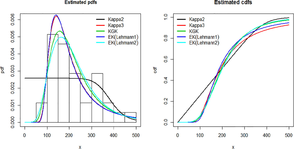
Plot of estimated pdf and cdf for stream flow amounts.

9 Conclusion

In this paper, we propose a five-parameter Kumaraswamy generalized Kappa distribution. Algebraic expressions for various properties of the proposed distribution are provided. The method of maximum likelihood is employed to estimate the parameters along with an empirical illustration expressing the application by using stream flow amount data set. The proposed distribution is compared with some similar existing distributions by using Cramer-von Mises $(W^{*})$ and Anderson-Darling $(A^{*})$ statistics as measure of goodness of fit. It is concluded that KGK distribution is good competitive model for stream flow data set. The proposed distribution KGK has the potential to attract wider application in various areas such as hydrology, reliability and survival analysis.

Acknowledgment

The authors are grateful to the anonymous learned reviewers for their valuable suggestions which have greatly helped in improving the presentation of the manuscript.

References

Alexander C., Cordeiro G.M., Ortega E.M.M., Sarabia J.M., . Generalized beta-generated distributions. Comput. Stat. Data Anal.. 2012;56(6):1880-1897.
[CrossRef] [Google Scholar]
Amini M., MirMostafaee S.M.T.K., Ahmadi J., . Log-gamma-generated families of distributions. Statistics. 2014;48(4):913-932.
[CrossRef] [Google Scholar]
Atkinson A.B., . On the measurement of th inequality. J. Econ. Theory. 1970;2(3):244-263.
[CrossRef] [Google Scholar]
Bonferroni C.E., . Elementi Di Statistica Generale. Firenze: Libreria Seeber; 1930.
Bourguignon M., Silva R.B., Cordeiro G.M., . The Weibull-G family of probability distributions. J. Data Sci.. 2014;12(1):53-68. www.jds-online.com/files/JDS-1210.pdf·2013-10-21
[Google Scholar]
Cordeiro G.M., de Castro M., . A new family of generalized distributions. J. Stat. Comput. Simul.. 2011;81(7):883-898.
[CrossRef] [Google Scholar]
Cordeiro G.M., Ortega E.M.M., da Cunha D.C.C., . The exponentiated generalized class of distributions. J. Data Sci.. 2013;11(1):1-27.
[Google Scholar]
Cowell F.A., . On the structure of additive inequality measures. Rev. Econ. Stud.. 1980;47(3):521-531. Oxford University Press
[Google Scholar]
Eugene N., Lee C., Famoye F., . Beta-normal distribution and its applications. Commun. Statist. Theory Methods. 2002;31(4):497-512.
[CrossRef] [Google Scholar]
Gini, C., 1914. Sulla Misura della concentrazione e della variabilit’a dei caratteri. Attidel regio Istituto Venteto di SS. LL.AA.,a.a. 1913-14, tomo LXXIII, parte II, pp. 1203–1248.
Gupta R.C., Gupta P.I., Gupta R.D., . Modeling failure time data by Lehmann alternatives. Commun. Statist. Theory Methods. 1998;27(4):887-904.
[CrossRef] [Google Scholar]
Gupta R.D., Kundu D., . Generalized exponential distribution. Austral. New Zealand J. Statist.. 1999;41(2):173-188.
[CrossRef] [Google Scholar]
Havrda J., Charvát F., . Quantification method in classification processes: concept of structural alpha-entropy. Kybernetika. 1967;3(1):30-35.
[Google Scholar]
Hussain, S., 2015. Properties, Extension and Application of Kappa Distribution. Unpublished M.Phil thesis submitted to Government College University, Faisalabad, Pakistan.
Jones M.C., . Families of distributions arising from the distributions of order statistics. Test. 2004;13(1):1-43.
[CrossRef] [Google Scholar]
Kumaraswamy P., . A generalized probability density function for double-bounded random processes. J. Hydrol.. 1980;46(1–2):79-88.
[CrossRef] [Google Scholar]
Lorenz M.O., . Methods of measuring the concentration of wealth. Publ. Am. Statist. Assoc.. 1905;9(70):209-219.
[CrossRef] [Google Scholar]
Marshall A.W., Olkin I., . A new method for adding a parameter to a family of distributions with applications to the exponential and weibull families. Biometrika. 1997;84(3):641-652.
[CrossRef] [Google Scholar]
Mielke P.W. Jr., . Another family of distributions for describing and analyzing precipitation data. J. Appl. Meteorol.. 1973;12(2):275-280.
[Google Scholar]
Mielke P.W., Johnson E.S., . Three parameter Kappa distribution maximum likelihood estimations and likelihood ratio tests. Monthly Weather Rev.. 1973;101:701-707. ftp://ftp.library.noaa.gov/docs.lib/htdocs/rescue/mwr/101/mwr-101-09-0701.pdf
[Google Scholar]
Pietra, G., 1915. Delle relazioni tra indici di variabilità, note I e II. Atti del Reale Istituto Veneto di Scienze, Lett ere ed Arti, a.a. 1914–15, LXXIV, 775–804.
Rényi A., . On Measures of Entropy and Information. University of California Press 1961:547-561.
[Google Scholar]
Ristic M.M., Balakrishnan N., . The gamma-exponentiated exponential distribution. J. Statist. Comput. Simul.. 2012;82(8):1191-1206.
[CrossRef] [Google Scholar]
Shorrocks A.F., . The class of additively decomposable inequality measures. Econometrica. 1980;48(3):613-625.
[Google Scholar]
Tsallis C., . Possible generalization of Boltzmann-Gibbs statistics. J. Statist. Phys.. 1988;52(1–2):479-487.
[CrossRef] [Google Scholar]
Zenga, M., 1984. Proposta per un indice di concentrazione basto sui rapporti fraquantili di populizone e quantili di reddito. Giornale degli Economisti e Annali di Economia Nuova Serie, Anno 43, No. 5/6 (Maggio-Giugno 1984), pp. 301–326. http://www.jstor.org/stable/23246074.
Zenga M., . Concentration curves and concentration indexes derived from them. In: Dagum C., Zenga M., eds. Income and Wealth Distribution, Inequality and Poverty. Studies in Contemporary Economics. Berlin, Heidelberg: Springer; 1990. p. :94-110.
[Google Scholar]
Zografos K., Balakrishnan N., . On families of beta- and generalized gamma-generated distributions and associated inference. Statist. Method.. 2009;6(4):344-362.
[CrossRef] [Google Scholar]

Appendix A

The elements of the $5 \times 5$ observed information matrix $J (Θ) = {U_{s, t}}$ where $s, t = a, b, α, β, θ$ are given by $U_{aa} = - \frac{n}{a^{2}} + (1 - b) \sum_{i = 1}^{n} \frac{{{logZ}_{i}}^{2}}{Z_{i}^{a} {[Z_{i}^{- a} - 1]}^{2}}, U_{ab} = - \sum_{i = 1}^{n} \frac{{logZ}_{i}}{Z_{i}^{- a} - 1}$ $U_{a α} = \frac{1}{α^{2}} \sum_{i = 1}^{n} \log [α + {(\frac{x_{i}}{β})}^{α θ}] - \frac{1}{α} \sum_{i = 1}^{n} {[α + {(\frac{x_{i}}{β})}^{α θ}]}^{- 1} - \frac{θ}{α} \sum_{i = 1}^{n} Z_{i}^{α} \log (\frac{x_{i}}{β}) + a (1 - b) \times \sum_{i = 1}^{n} {[Z_{i}^{- a} - 1]}^{- 2} Z_{i}^{- a - 1} Z_{i α}^{'} {logZ}_{i} + (1 - b) \sum_{i = 1}^{n} {[Z_{i}^{- a} - 1]}^{- 1} Z_{i}^{- 1} Z_{i α}^{'}$ $U_{a β} = \frac{θ}{β} [\sum_{i = 1}^{n} Z_{i}^{α} - n] + a (1 - b) \sum_{i = 1}^{n} {[Z_{i}^{- a} - 1]}^{- 2} Z_{i}^{- a - 1} Z_{i β}^{'} {logZ}_{i} + (1 - b) \sum_{i = 1}^{n} {[Z_{i}^{- a} - 1]}^{- 1} Z_{i}^{- 1} Z_{i β}^{'}$ $U_{a θ} = - nlog β + \sum_{i = 1}^{n} {logx}_{i} - \sum_{i = 1}^{n} Z_{i}^{α} \log (\frac{x_{i}}{β}) + a (1 - b) \times \sum_{i = 1}^{n} {[Z_{i}^{- a} - 1]}^{- 2} Z_{i}^{- a - 1} Z_{i θ}^{'} {logZ}_{i} + (1 - b) \sum_{i = 1}^{n} {[Z_{i}^{- a} - 1]}^{- 1} Z_{i}^{- 1} Z_{i θ}^{'}$ $U_{bb} = - \frac{n}{b^{2}}, U_{b α} = - a \sum_{i = 1}^{n} Z_{i}^{a - 1} Z_{i α}^{'} {[1 - Z_{i}^{a}]}^{- 1}, U_{b β} = - a \sum_{i = 1}^{n} Z_{i}^{a - 1} Z_{i β}^{'} {[1 - Z_{i}^{a}]}^{- 1} U_{b θ} = - a \sum_{i = 1}^{n} Z_{i}^{a - 1} Z_{i θ}^{'} {[1 - Z_{i}^{a}]}^{- 1}$ $U_{α α} = - \frac{n}{α^{2}} - \frac{2 a}{α^{3}} \sum_{i = 1}^{n} \log [α + {(\frac{x_{i}}{β})}^{α θ}] + \frac{2 a}{α^{2}} \sum_{i = 1}^{n} {[α + {(\frac{x_{i}}{β})}^{α θ}]}^{- 1} + \frac{a}{α^{2}} \sum_{i = 1}^{n} θ Z_{i}^{α} \log (\frac{x_{i}}{β}) + (1 + \frac{a}{α}) \sum_{i = 1}^{n} {[α + {(\frac{x_{i}}{β})}^{α θ}]}^{- 2} + (1 + \frac{a}{α}) \sum_{i = 1}^{n} θ Z_{i}^{2 α} {(\frac{x_{i}}{β})}^{- α θ} \log (\frac{x_{i}}{β}) + \frac{a θ}{α^{2}} \times \sum_{i = 1}^{n} Z_{i}^{α} \log (\frac{x_{i}}{β}) - θ (1 + \frac{a}{α}) \sum_{i = 1}^{n} [Z_{i}^{α} {logZ}_{i} + α Z_{i}^{α - 1} Z_{i α}^{'}] \log (\frac{x_{i}}{β}) + a (1 - b) \sum_{i = 1}^{n} [\frac{(1 - Z_{i}^{a}) {Z_{i}^{a - 1} Z_{i α}^{″} + (a - 1) Z_{i}^{a - 2} {(Z_{i α}^{'})}^{2}} + {aZ}_{i}^{2 a - 2} {(Z_{i α}^{'})}^{2}}{{(1 - Z_{i}^{a})}^{2}}]$ $U_{α β} = - \frac{a θ}{α β} \sum_{i = 1}^{n} Z_{i}^{α} - \frac{(a + α) θ}{β} \sum_{i = 1}^{n} Z_{i}^{2 α} {(\frac{x_{i}}{β})}^{- α θ} - (a + θ) \sum_{i = 1}^{n} [α Z_{i}^{α - 1} Z_{i β}^{'} \log (\frac{x_{i}}{β}) - \frac{Z_{i}^{α}}{β}] + a (1 - b) \sum_{i = 1}^{n} [\frac{(1 - Z_{i}^{a}) \{Z_{i}^{a - 1} Z_{i α β}^{″} + (a - 1) Z_{i}^{a - 2} Z_{i α}^{'} Z_{i β}^{'}\} + {aZ}_{i}^{2 a - 2} Z_{i α}^{'} Z_{i β}^{'}}{{(1 - Z_{i}^{a})}^{2}}]$ $U_{α θ} = (a + α) \sum_{i = 1}^{n} Z_{i}^{2 α} {(\frac{x_{i}}{β})}^{- α θ} \log (\frac{x_{i}}{β}) - \sum_{i = 1}^{n} Z_{i}^{α} \log (\frac{x_{i}}{β}) - θ (a + α) u m_{i = 1}^{n} Z_{i}^{α - 1} Z_{i θ}^{'} \log (\frac{x_{i}}{β}) + a (1 - b) \sum_{i = 1}^{n} [\frac{(1 - Z_{i}^{a}) {Z_{i}^{a - 1} Z_{i α θ}^{″} + (a - 1) Z_{i}^{a - 2} Z_{i α}^{'} Z_{i θ}^{'}} + {aZ}_{i}^{2 a - 2} Z_{i α}^{'} Z_{i θ}^{'}}{{(1 - Z_{i}^{a})}^{2}}]$ $U_{β β} = \frac{na θ}{β^{2}} - \frac{(a + α) θ}{β^{2}} \sum_{i = 1}^{n} Z_{i}^{α} + \frac{α θ (a + α)}{β} \sum_{i = 1}^{n} Z_{i}^{α - 1} Z_{i β}^{'} + a (1 - b) \sum_{i = 1}^{n} [\frac{(1 - Z_{i}^{a}) {Z_{i}^{a - 1} Z_{i β}^{″} + (a - 1) Z_{i}^{a - 2} {(Z_{i β}^{'})}^{2}} + {aZ}_{i}^{2 a - 2} {(Z_{i β}^{'})}^{2}}{{(1 - Z_{i}^{a})}^{2}}]$ $U_{β θ} = - \frac{na}{β} + \frac{(a + α)}{β} \sum_{i = 1}^{n} Z_{i}^{α} + \frac{α θ (a + α)}{β} \sum_{i = 1}^{n} Z_{i}^{α - 1} Z_{i θ}^{'} + a (1 - b) \sum_{i = 1}^{n} [\frac{(1 - Z_{i}^{a}) {Z_{i}^{a - 1} Z_{i β θ}^{″} + (a - 1) Z_{i}^{a - 2} Z_{i β}^{'} Z_{i θ}^{'}} + {aZ}_{i}^{2 a - 2} Z_{i β}^{'} Z_{i θ}^{'}}{{(1 - Z_{i}^{a})}^{2}}]$ $U_{θ θ} = - \frac{n}{θ^{2}} (1 - a θ \log β) - \frac{na}{θ} \log β - α (a + α) \sum_{i = 1}^{n} Z_{i}^{α - 1} Z_{i θ}^{'} \log (\frac{x_{i}}{β}) + a (1 - b) \sum_{i = 1}^{n} [\frac{(1 - Z_{i}^{a}) {Z_{i}^{a - 1} Z_{i θ}^{″} + (a - 1) Z_{i}^{a - 2} {(Z_{i θ}^{'})}^{2}} + {aZ}_{i}^{2 a - 2} {(Z_{i θ}^{'})}^{2}}{{(1 - Z_{i}^{a})}^{2}}]$ where $Z_{i α}^{'} = \frac{1}{α^{2}} Z_{i} \log [α + {(\frac{x_{i}}{β})}^{α θ}] - \frac{1}{α} Z_{i}^{α + 1} {(\frac{x_{i}}{β})}^{- α θ} - \frac{θ}{α} Z_{i}^{α + 1} \log (\frac{x_{i}}{β})$ $Z_{i β}^{'} = \frac{θ}{β} {Z_{i}^{α + 1} - Z_{i}}$ $Z_{i θ}^{'} = \log (\frac{x_{i}}{β}) [Z_{i} - Z_{i}^{α + 1}]$ $Z_{i α}^{″} = \{{(\frac{x_{i}}{β})}^{- α θ} + θ \log (\frac{x_{i}}{β})\} [\frac{2}{α^{2}} Z_{i}^{α + 1} - (1 + \frac{1}{α}) Z_{i}^{α} Z_{i α}^{'} - \frac{1}{α} Z_{i}^{α + 1} {logZ}_{i}] + [\frac{Z_{i α}^{'}}{α^{2}} - \frac{2}{α^{3}} Z_{i}] \log [α + {(\frac{x_{i}}{β})}^{α θ}] + \frac{θ}{α} Z_{i}^{α + 1} {(\frac{x_{i}}{β})}^{- α θ} \log (\frac{x_{i}}{β})$ $Z_{i α β}^{″} = \frac{1}{α^{2}} Z_{i β}^{'} \log [α + {(\frac{x_{i}}{β})}^{α θ}] - \frac{θ}{β} Z_{i}^{α + 1} {(\frac{x_{i}}{β})}^{- α θ} - (1 + \frac{1}{α}) Z_{i}^{α} Z_{i β}^{'} \times [{(\frac{x_{i}}{β})}^{- α θ} + θ \log (\frac{x_{i}}{β})]$ $Z_{i α θ}^{″} = \frac{1}{α^{2}} Z_{i θ}^{'} \log [α + {(\frac{x_{i}}{β})}^{α θ}] + \frac{θ}{α} Z_{i}^{α + 1} {(\frac{x_{i}}{β})}^{- α θ} \log (\frac{x_{i}}{β}) - (1 + \frac{1}{α}) Z_{i}^{α} Z_{i θ}^{'} [{(\frac{x_{i}}{β})}^{- α θ} + θ \log (\frac{x_{i}}{β})]$ $Z_{i β}^{″} = \frac{θ}{β^{2}} Z_{i} [1 - Z_{i}^{α}] + \frac{θ}{β} Z_{i β}^{'} [(α + 1) Z_{i}^{α} - 1]$ $Z_{i β θ}^{″} = \frac{1}{β} [Z_{i}^{α + 1} + θ (α + 1) Z_{i}^{α} Z_{i θ}^{'} + θ Z_{i θ}^{'} + Z_{i}]$ $Z_{i θ}^{″} = \log (\frac{x_{i}}{β}) Z_{i θ}^{'} [1 - (α + 1) Z_{i}^{α}]$

Show Sections

[1] Alexander C., Cordeiro G.M., Ortega E.M.M., Sarabia J.M., . Generalized beta-generated distributions. Comput. Stat. Data Anal.. 2012;56(6):1880-1897.
[CrossRef] [Google Scholar]

[2] Amini M., MirMostafaee S.M.T.K., Ahmadi J., . Log-gamma-generated families of distributions. Statistics. 2014;48(4):913-932.
[CrossRef] [Google Scholar]

[3] Atkinson A.B., . On the measurement of th inequality. J. Econ. Theory. 1970;2(3):244-263.
[CrossRef] [Google Scholar]

[4] Bonferroni C.E., . Elementi Di Statistica Generale. Firenze: Libreria Seeber; 1930.

[5] Bourguignon M., Silva R.B., Cordeiro G.M., . The Weibull-G family of probability distributions. J. Data Sci.. 2014;12(1):53-68. www.jds-online.com/files/JDS-1210.pdf·2013-10-21
[Google Scholar]

[6] Cordeiro G.M., de Castro M., . A new family of generalized distributions. J. Stat. Comput. Simul.. 2011;81(7):883-898.
[CrossRef] [Google Scholar]

[7] Cordeiro G.M., Ortega E.M.M., da Cunha D.C.C., . The exponentiated generalized class of distributions. J. Data Sci.. 2013;11(1):1-27.
[Google Scholar]

[8] Cowell F.A., . On the structure of additive inequality measures. Rev. Econ. Stud.. 1980;47(3):521-531. Oxford University Press
[Google Scholar]

[9] Eugene N., Lee C., Famoye F., . Beta-normal distribution and its applications. Commun. Statist. Theory Methods. 2002;31(4):497-512.
[CrossRef] [Google Scholar]

[10] Gini, C., 1914. Sulla Misura della concentrazione e della variabilit’a dei caratteri. Attidel regio Istituto Venteto di SS. LL.AA.,a.a. 1913-14, tomo LXXIII, parte II, pp. 1203–1248.

[11] Gupta R.C., Gupta P.I., Gupta R.D., . Modeling failure time data by Lehmann alternatives. Commun. Statist. Theory Methods. 1998;27(4):887-904.
[CrossRef] [Google Scholar]

[12] Gupta R.D., Kundu D., . Generalized exponential distribution. Austral. New Zealand J. Statist.. 1999;41(2):173-188.
[CrossRef] [Google Scholar]

[13] Havrda J., Charvát F., . Quantification method in classification processes: concept of structural alpha-entropy. Kybernetika. 1967;3(1):30-35.
[Google Scholar]

[14] Hussain, S., 2015. Properties, Extension and Application of Kappa Distribution. Unpublished M.Phil thesis submitted to Government College University, Faisalabad, Pakistan.

[15] Jones M.C., . Families of distributions arising from the distributions of order statistics. Test. 2004;13(1):1-43.
[CrossRef] [Google Scholar]

[16] Kumaraswamy P., . A generalized probability density function for double-bounded random processes. J. Hydrol.. 1980;46(1–2):79-88.
[CrossRef] [Google Scholar]

[17] Lorenz M.O., . Methods of measuring the concentration of wealth. Publ. Am. Statist. Assoc.. 1905;9(70):209-219.
[CrossRef] [Google Scholar]

[18] Marshall A.W., Olkin I., . A new method for adding a parameter to a family of distributions with applications to the exponential and weibull families. Biometrika. 1997;84(3):641-652.
[CrossRef] [Google Scholar]

[19] Mielke P.W. Jr., . Another family of distributions for describing and analyzing precipitation data. J. Appl. Meteorol.. 1973;12(2):275-280.
[Google Scholar]

[20] Mielke P.W., Johnson E.S., . Three parameter Kappa distribution maximum likelihood estimations and likelihood ratio tests. Monthly Weather Rev.. 1973;101:701-707. ftp://ftp.library.noaa.gov/docs.lib/htdocs/rescue/mwr/101/mwr-101-09-0701.pdf
[Google Scholar]

[21] Pietra, G., 1915. Delle relazioni tra indici di variabilità, note I e II. Atti del Reale Istituto Veneto di Scienze, Lett ere ed Arti, a.a. 1914–15, LXXIV, 775–804.

[22] Rényi A., . On Measures of Entropy and Information. University of California Press 1961:547-561.
[Google Scholar]

[23] Ristic M.M., Balakrishnan N., . The gamma-exponentiated exponential distribution. J. Statist. Comput. Simul.. 2012;82(8):1191-1206.
[CrossRef] [Google Scholar]

[24] Shorrocks A.F., . The class of additively decomposable inequality measures. Econometrica. 1980;48(3):613-625.
[Google Scholar]

[25] Tsallis C., . Possible generalization of Boltzmann-Gibbs statistics. J. Statist. Phys.. 1988;52(1–2):479-487.
[CrossRef] [Google Scholar]

[26] Zenga, M., 1984. Proposta per un indice di concentrazione basto sui rapporti fraquantili di populizone e quantili di reddito. Giornale degli Economisti e Annali di Economia Nuova Serie, Anno 43, No. 5/6 (Maggio-Giugno 1984), pp. 301–326. http://www.jstor.org/stable/23246074.

[27] Zenga M., . Concentration curves and concentration indexes derived from them. In: Dagum C., Zenga M., eds. Income and Wealth Distribution, Inequality and Poverty. Studies in Contemporary Economics. Berlin, Heidelberg: Springer; 1990. p. :94-110.
[Google Scholar]

[28] Zografos K., Balakrishnan N., . On families of beta- and generalized gamma-generated distributions and associated inference. Statist. Method.. 2009;6(4):344-362.
[CrossRef] [Google Scholar]

Kumaraswamy generalized Kappa distribution with application to stream flow data

Abstract

Keywords

Entropy

Inequality indices

Kumaraswamy distribution

Kappa distribution

Maximum likelihood

1 Introduction

2 Kumaraswamy generalized Kappa distribution

2.1 Special sub-models

2.2 A useful representation of KGK density function

3 Statistical properties

3.1 Quantile function and random number generation

3.2 Mode

3.3 rth moment

3.4 Moment generating function and characteristic function

4 Reliability properties

5 Inequality measures

5.1 Gini index

5.2 Lorenz curve

5.3 Bonferroni curve

5.4 Zenga index

5.5 Atkinson index

5.6 Pietra index

5.7 Generalized entropy (GE)

6 Entropies

6.1 Rényi entropy

6.2 β -entropy

7 Estimation of parameters of KGK distribution

8 Empirical illustration

9 Conclusion

Acknowledgment

References

Appendix A

Suggested read for related articles:

6.2 $β$ -entropy